Radon变换

在计算机层析成像中，层析重建问题是从一组投影中获得层析切片图像 1. 投影是通过绘制一组穿过感兴趣的2D对象的平行光线，将对象沿每条光线的对比度的积分分配给投影中的单个像素来形成的。2D对象的单个投影是一维的。为了能够对对象进行计算机断层扫描重建，必须获取多个投影，每个投影对应于射线相对于对象的不同角度。几个角度的投影的集合称为正弦图，它是原始图像的线性变换。

逆Radon变换在计算机层析成像中用于从测量的投影(正弦图)重建2D图像。逆Radon变换并不存在一个实用的、准确的实现，但有几个好的近似算法可用。

当逆Radon变换从一组投影重建对象时，(正)Radon变换可用于模拟层析实验。

该脚本执行Radon变换以模拟层析实验，并基于模拟形成的结果正弦图重建输入图像。比较了两种实现Radon逆变换和重建原始图像的方法：滤波反投影法(FBP)和同时代数重建技术(SART)。

有关层析重建的更多信息，请参见

1(1,2)

M·斯兰尼，《计算机断层成像原理》，IEEE出版社，1988。Http://www.slaney.org/pct/pct-toc.html

2

维基百科、Radon变换、https://en.wikipedia.org/wiki/Radon_transform#Relationship_with_the_Fourier_transform

3(1,2)

S Kaczmarz，《Angenaeherte Auflesung von Systens Lineer Gleichugen》，《Polonaise de Science et des Lettres》，35页，第355-357页(1937)

4

Ah Andersen，AC Kak，“同步代数重建技术(SART)：ART算法的卓越实现”，超声成像6页81-94(1984)

正向变换

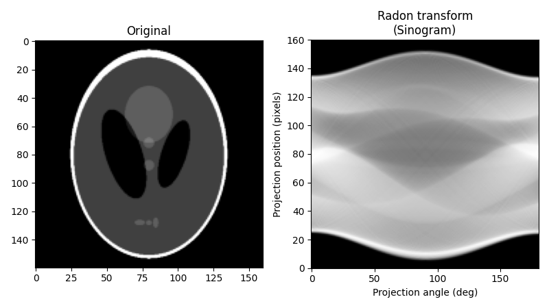
作为我们的原始图像，我们将使用谢普-洛根模型。在计算Radon变换时，我们需要确定要使用多少个投影角。根据经验，投影的数量应该与对象上存在的像素数量大致相同(要了解为什么会这样，请考虑在重建过程中必须确定多少未知像素值，并将其与投影提供的测量值进行比较)，我们在这里遵循这一规则。下面是原始图像及其Radon变换，通常称为其 正弦图形 ：

import numpy as np
import matplotlib.pyplot as plt

from skimage.data import shepp_logan_phantom
from skimage.transform import radon, rescale

image = shepp_logan_phantom()
image = rescale(image, scale=0.4, mode='reflect', multichannel=False)

fig, (ax1, ax2) = plt.subplots(1, 2, figsize=(8, 4.5))

ax1.set_title("Original")
ax1.imshow(image, cmap=plt.cm.Greys_r)

theta = np.linspace(0., 180., max(image.shape), endpoint=False)
sinogram = radon(image, theta=theta, circle=True)
dx, dy = 0.5 * 180.0 / max(image.shape), 0.5 / sinogram.shape[0]
ax2.set_title("Radon transform\n(Sinogram)")
ax2.set_xlabel("Projection angle (deg)")
ax2.set_ylabel("Projection position (pixels)")
ax2.imshow(sinogram, cmap=plt.cm.Greys_r,
           extent=(-dx, 180.0 + dx, -dy, sinogram.shape[0] + dy),
           aspect='auto')

fig.tight_layout()
plt.show()

输出：

/scikit-image/doc/examples/transform/plot_radon_transform.py:69: FutureWarning:

`multichannel` is a deprecated argument name for `rescale`. It will be removed in version 1.0. Please use `channel_axis` instead.

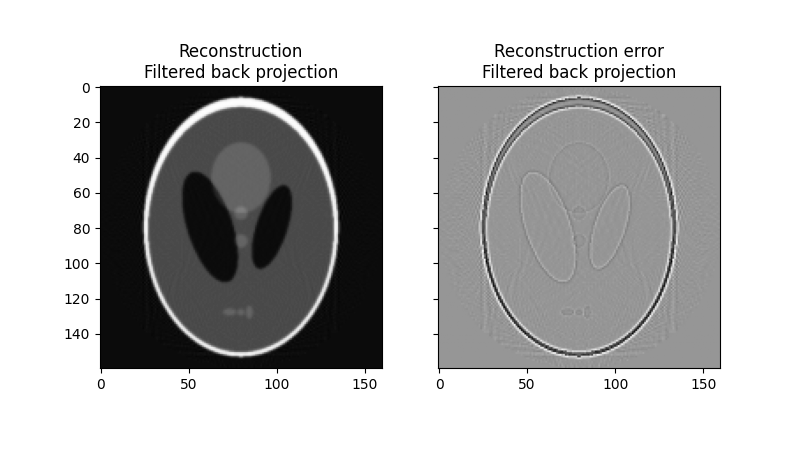
滤波反投影法(FBP)重建

滤波反投影的数学基础是傅里叶切片定理 2. 它利用傅里叶投影的傅里叶变换和傅里叶空间的内插得到图像的二维傅立叶变换，然后进行逆变换形成重建图像。滤波反投影法是执行反Radon变换的最快方法之一。FBP的唯一可调参数是应用于傅里叶变换投影的过滤器。它可以用来抑制重建过程中的高频噪声。 skimage 为滤镜提供了几个不同的选项。

from skimage.transform import iradon

reconstruction_fbp = iradon(sinogram, theta=theta, circle=True)
error = reconstruction_fbp - image
print(f"FBP rms reconstruction error: {np.sqrt(np.mean(error**2)):.3g}")

imkwargs = dict(vmin=-0.2, vmax=0.2)
fig, (ax1, ax2) = plt.subplots(1, 2, figsize=(8, 4.5),
                               sharex=True, sharey=True)
ax1.set_title("Reconstruction\nFiltered back projection")
ax1.imshow(reconstruction_fbp, cmap=plt.cm.Greys_r)
ax2.set_title("Reconstruction error\nFiltered back projection")
ax2.imshow(reconstruction_fbp - image, cmap=plt.cm.Greys_r, **imkwargs)
plt.show()

输出：

FBP rms reconstruction error: 0.0283

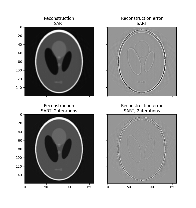
基于同时代数重构技术的重构

用于层析成像的代数重建技术基于一个简单的想法：对于像素化的图像，特定投影中的单条射线的值仅仅是该射线在穿过对象的途中通过的所有像素的总和。这是一种表示正向Radon变换的方式。然后，逆Radon变换可以表示为一组(大的)线性方程。当每条光线穿过图像中的一小部分像素时，这组方程是稀疏的，允许稀疏线性系统的迭代解算器处理方程系统。有一种迭代方法特别流行，那就是Kaczmarz方法 3, 它具有解将逼近方程组的最小二乘解的性质。

将重建问题表述为一组线性方程和迭代求解器的组合使代数技术相对灵活，因此可以相对容易地结合某些形式的先验知识。

skimage 提供了一种比较流行的代数重建技术：同时代数重建技术(SART) 1 4 。它使用Kaczmarz的方法 3 作为迭代求解器。良好的重建通常在一次迭代中获得，这使得该方法在计算上是有效的。运行一个或多个额外的迭代通常会改进尖锐的高频特征的重建，并以增加的高频噪声为代价降低均方误差(用户将需要决定什么迭代次数最适合手头的问题)。中的实现 skimage 允许将关于重建值的下限阈值和上限阈值的形式的先验信息提供给重建。

from skimage.transform import iradon_sart

reconstruction_sart = iradon_sart(sinogram, theta=theta)
error = reconstruction_sart - image
print("SART (1 iteration) rms reconstruction error: "
      f"{np.sqrt(np.mean(error**2)):.3g}")

fig, axes = plt.subplots(2, 2, figsize=(8, 8.5), sharex=True, sharey=True)
ax = axes.ravel()

ax[0].set_title("Reconstruction\nSART")
ax[0].imshow(reconstruction_sart, cmap=plt.cm.Greys_r)

ax[1].set_title("Reconstruction error\nSART")
ax[1].imshow(reconstruction_sart - image, cmap=plt.cm.Greys_r, **imkwargs)

# Run a second iteration of SART by supplying the reconstruction
# from the first iteration as an initial estimate
reconstruction_sart2 = iradon_sart(sinogram, theta=theta,
                                   image=reconstruction_sart)
error = reconstruction_sart2 - image
print("SART (2 iterations) rms reconstruction error: "
      f"{np.sqrt(np.mean(error**2)):.3g}")

ax[2].set_title("Reconstruction\nSART, 2 iterations")
ax[2].imshow(reconstruction_sart2, cmap=plt.cm.Greys_r)

ax[3].set_title("Reconstruction error\nSART, 2 iterations")
ax[3].imshow(reconstruction_sart2 - image, cmap=plt.cm.Greys_r, **imkwargs)
plt.show()

输出：

SART (1 iteration) rms reconstruction error: 0.0329
SART (2 iterations) rms reconstruction error: 0.0214