评估细分指标

当尝试不同的分割方法时，你如何知道哪种方法最好？如果你有一个 基本事实 或 金本位 分段，您可以使用各种度量来检查每个自动化方法与事实的接近程度。在这个例子中，我们使用一个容易分割的图像作为如何解释各种分割度量的例子。我们将使用适应的兰德误差和信息的变化作为示例度量，并了解如何 过度细分 (将真实分段拆分成太多的子分段)和 细分不足 (将不同的真实分段合并为一个分段)会影响不同的分数。

import numpy as np
import matplotlib.pyplot as plt
from scipy import ndimage as ndi

from skimage import data
from skimage.metrics import (adapted_rand_error,
                              variation_of_information)
from skimage.filters import sobel
from skimage.measure import label
from skimage.util import img_as_float
from skimage.feature import canny
from skimage.morphology import remove_small_objects
from skimage.segmentation import (morphological_geodesic_active_contour,
                                  inverse_gaussian_gradient,
                                  watershed,
                                  mark_boundaries)

image = data.coins()

首先，我们生成真正的分割。对于这个简单的图像，我们知道精确的函数和参数，这些函数和参数将产生完美的分割。在真实场景中，您通常会通过手动注释或对分段进行“绘制”来生成基本事实。

elevation_map = sobel(image)
markers = np.zeros_like(image)
markers[image < 30] = 1
markers[image > 150] = 2
im_true = watershed(elevation_map, markers)
im_true = ndi.label(ndi.binary_fill_holes(im_true - 1))[0]

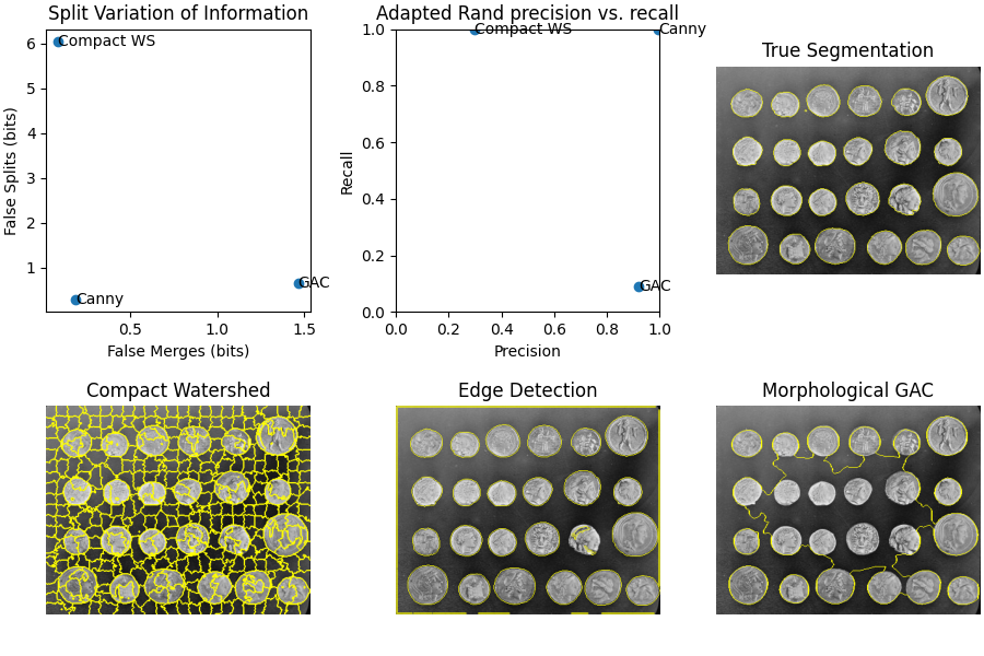
接下来，我们创建三个具有不同特征的不同分段。第一个使用 skimage.segmentation.watershed() 使用 紧凑性 ，这是一个有用的初始分割，但作为最终结果太细了。我们将看到这如何导致过度细分指标激增。

edges = sobel(image)
im_test1 = watershed(edges, markers=468, compactness=0.001)

下一种方法使用坎尼边缘滤波器， skimage.filters.canny() 。这是一个非常好的边缘搜索器，并给出了平衡的结果。

edges = canny(image)
fill_coins = ndi.binary_fill_holes(edges)
im_test2 = ndi.label(remove_small_objects(fill_coins, 21))[0]

最后，我们使用形态测地线活动轮廓， skimage.segmentation.morphological_geodesic_active_contour() ，这种方法通常会产生很好的结果，但需要很长时间才能收敛到一个好的答案。我们有意将该过程缩短为100次迭代，因此最终结果为 分段不足 这意味着许多地区被合并到一个分段中。我们将看到对细分指标的相应影响。

image = img_as_float(image)
gradient = inverse_gaussian_gradient(image)
init_ls = np.zeros(image.shape, dtype=np.int8)
init_ls[10:-10, 10:-10] = 1
im_test3 = morphological_geodesic_active_contour(gradient, iterations=100,
                                                 init_level_set=init_ls,
                                                 smoothing=1, balloon=-1,
                                                 threshold=0.69)
im_test3 = label(im_test3)

method_names = ['Compact watershed', 'Canny filter',
                'Morphological Geodesic Active Contours']
short_method_names = ['Compact WS', 'Canny', 'GAC']

precision_list = []
recall_list = []
split_list = []
merge_list = []
for name, im_test in zip(method_names, [im_test1, im_test2, im_test3]):
    error, precision, recall = adapted_rand_error(im_true, im_test)
    splits, merges = variation_of_information(im_true, im_test)
    split_list.append(splits)
    merge_list.append(merges)
    precision_list.append(precision)
    recall_list.append(recall)
    print(f"\n## Method: {name}")
    print(f"Adapted Rand error: {error}")
    print(f"Adapted Rand precision: {precision}")
    print(f"Adapted Rand recall: {recall}")
    print(f"False Splits: {splits}")
    print(f"False Merges: {merges}")

fig, axes = plt.subplots(2, 3, figsize=(9, 6), constrained_layout=True)
ax = axes.ravel()

ax[0].scatter(merge_list, split_list)
for i, txt in enumerate(short_method_names):
    ax[0].annotate(txt, (merge_list[i], split_list[i]),
                   verticalalignment='center')
ax[0].set_xlabel('False Merges (bits)')
ax[0].set_ylabel('False Splits (bits)')
ax[0].set_title('Split Variation of Information')

ax[1].scatter(precision_list, recall_list)
for i, txt in enumerate(short_method_names):
    ax[1].annotate(txt, (precision_list[i], recall_list[i]),
                   verticalalignment='center')
ax[1].set_xlabel('Precision')
ax[1].set_ylabel('Recall')
ax[1].set_title('Adapted Rand precision vs. recall')
ax[1].set_xlim(0, 1)
ax[1].set_ylim(0, 1)

ax[2].imshow(mark_boundaries(image, im_true))
ax[2].set_title('True Segmentation')
ax[2].set_axis_off()

ax[3].imshow(mark_boundaries(image, im_test1))
ax[3].set_title('Compact Watershed')
ax[3].set_axis_off()

ax[4].imshow(mark_boundaries(image, im_test2))
ax[4].set_title('Edge Detection')
ax[4].set_axis_off()

ax[5].imshow(mark_boundaries(image, im_test3))
ax[5].set_title('Morphological GAC')
ax[5].set_axis_off()

plt.show()

输出：

/scikit-image/doc/examples/segmentation/plot_metrics.py:80: FutureWarning:

`iterations` is a deprecated argument name for `morphological_geodesic_active_contour`. It will be removed in version 1.0. Please use `num_iter` instead.


## Method: Compact watershed
Adapted Rand error: 0.5421684624091794
Adapted Rand precision: 0.2968781380256405
Adapted Rand recall: 0.9999664222191392
False Splits: 6.036024332525563
False Merges: 0.0825883711820654

## Method: Canny filter
Adapted Rand error: 0.0027247598212836177
Adapted Rand precision: 0.9946425605360896
Adapted Rand recall: 0.9999218934767155
False Splits: 0.29216655391322216
False Merges: 0.18066750731998152

## Method: Morphological Geodesic Active Contours
Adapted Rand error: 0.8346015951433162
Adapted Rand precision: 0.9191321393095933
Adapted Rand recall: 0.09087577915161697
False Splits: 0.6466330168716372
False Merges: 1.4656270133195097