洪泛填土

泛洪填充是一种基于图像中与初始种子点的相似性来识别和/或更改图像中相邻值的算法 1. 概念上的类比是许多图形编辑器中的“画桶”工具。

1

https://en.wikipedia.org/wiki/Flood_fill

基本示例

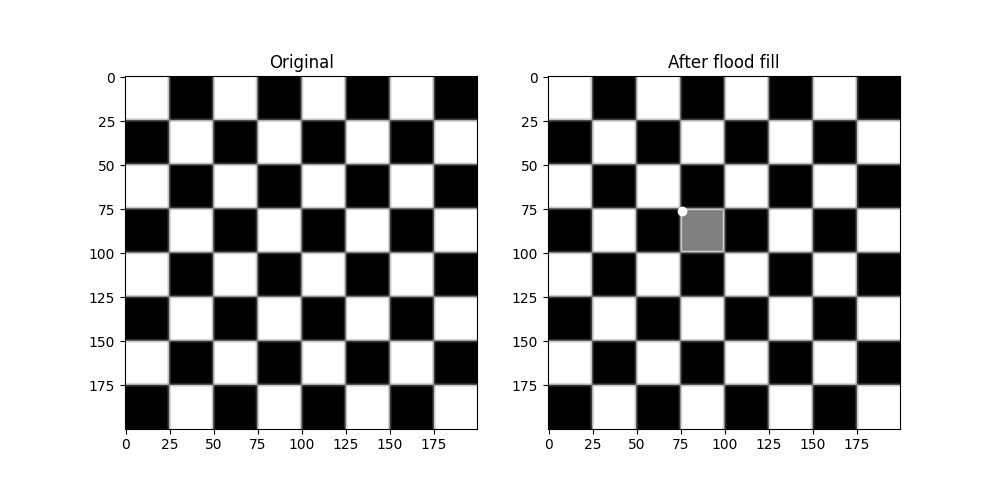
首先，我们将棋盘正方形从白色更改为中灰色的基本示例。

import numpy as np
import matplotlib.pyplot as plt
from skimage import data, filters, color, morphology
from skimage.segmentation import flood, flood_fill


checkers = data.checkerboard()

# Fill a square near the middle with value 127, starting at index (76, 76)
filled_checkers = flood_fill(checkers, (76, 76), 127)

fig, ax = plt.subplots(ncols=2, figsize=(10, 5))

ax[0].imshow(checkers, cmap=plt.cm.gray)
ax[0].set_title('Original')

ax[1].imshow(filled_checkers, cmap=plt.cm.gray)
ax[1].plot(76, 76, 'wo')  # seed point
ax[1].set_title('After flood fill')

plt.show()

高级范例

由于标准的洪水填充要求邻居严格相等，因此其使用仅限于具有颜色渐变和噪声的真实图像。这个 tolerance 关键字参数扩大了初始值的允许范围，允许在真实图像上使用。

在这里，我们将在摄影师身上做一点实验。首先，把他的外套从深色转成浅色。

cameraman = data.camera()

# Change the cameraman's coat from dark to light (255).  The seed point is
# chosen as (155, 150)
light_coat = flood_fill(cameraman, (155, 150), 255, tolerance=10)
fig, ax = plt.subplots(ncols=2, figsize=(10, 5))

ax[0].imshow(cameraman, cmap=plt.cm.gray)
ax[0].set_title('Original')
ax[0].axis('off')

ax[1].imshow(light_coat, cmap=plt.cm.gray)
ax[1].plot(150, 155, 'ro')  # seed point
ax[1].set_title('After flood fill')
ax[1].axis('off')

plt.show()

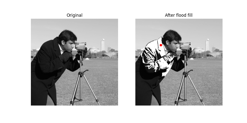
摄影师的外套是各种深浅不一的灰色。只有与种子值附近的阴影匹配的外套部分才会更改。

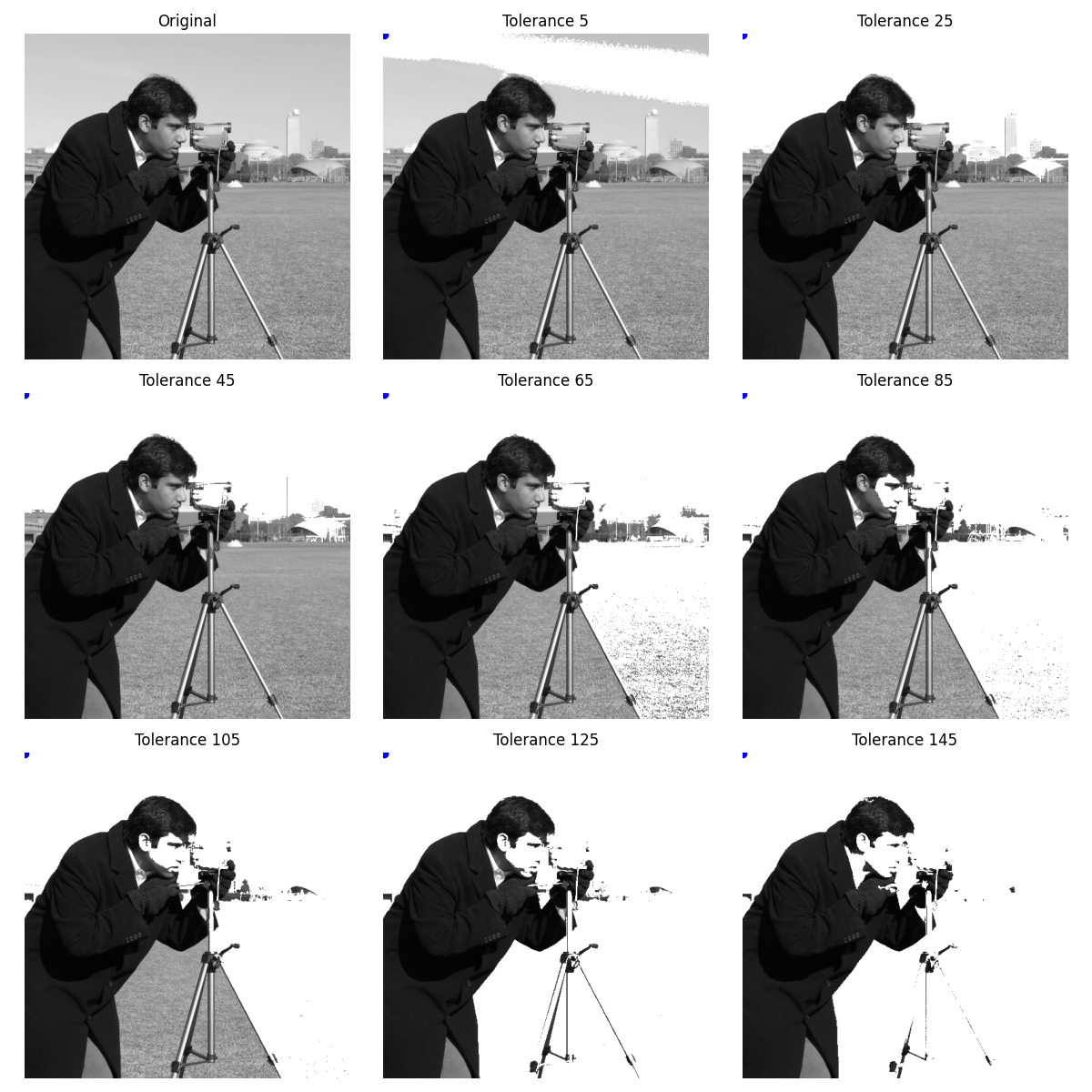
关于公差的实验

为了更直观地了解公差参数是如何工作的，这里有一组逐渐增加参数的图像，种子点位于左上角。

output = []

for i in range(8):
    tol = 5 + 20 * i
    output.append(flood_fill(cameraman, (0, 0), 255, tolerance=tol))

# Initialize plot and place original image
fig, ax = plt.subplots(nrows=3, ncols=3, figsize=(12, 12))
ax[0, 0].imshow(cameraman, cmap=plt.cm.gray)
ax[0, 0].set_title('Original')
ax[0, 0].axis('off')

# Plot all eight different tolerances for comparison.
for i in range(8):
    m, n = np.unravel_index(i + 1, (3, 3))
    ax[m, n].imshow(output[i], cmap=plt.cm.gray)
    ax[m, n].set_title('Tolerance {0}'.format(str(5 + 20 * i)))
    ax[m, n].axis('off')
    ax[m, n].plot(0, 0, 'bo')  # seed point

fig.tight_layout()
plt.show()

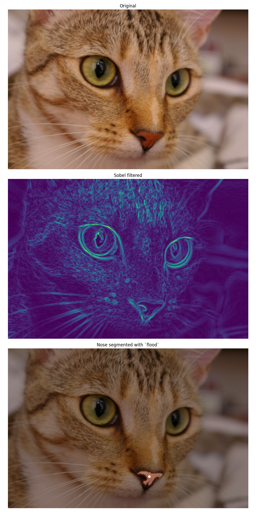
泛洪作为遮罩

一个姊妹功能， flood ，返回标识泛洪的遮罩，而不是修改图像本身。这对于分段和更高级的分析管道非常有用。

这里我们分割一只猫的鼻子。但是，整体应用不支持多通道图像 [_fill] 。取而代之的是，我们对红色通道进行Sobel过滤以增强边缘，然后用容差淹没鼻子。

cat = data.chelsea()
cat_sobel = filters.sobel(cat[..., 0])
cat_nose = flood(cat_sobel, (240, 265), tolerance=0.03)

fig, ax = plt.subplots(nrows=3, figsize=(10, 20))

ax[0].imshow(cat)
ax[0].set_title('Original')
ax[0].axis('off')

ax[1].imshow(cat_sobel)
ax[1].set_title('Sobel filtered')
ax[1].axis('off')

ax[2].imshow(cat)
ax[2].imshow(cat_nose, cmap=plt.cm.gray, alpha=0.3)
ax[2].plot(265, 240, 'wo')  # seed point
ax[2].set_title('Nose segmented with `flood`')
ax[2].axis('off')

fig.tight_layout()
plt.show()

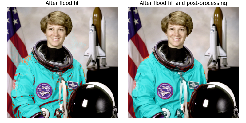
HSV空间充填和掩模后处理

由于泛洪填充是在单通道图像上操作的，因此我们在这里将图像变换到HSV(色调饱和值)空间，以便泛洪具有相似色调的像素。

在此示例中，我们还说明可以后处理由 skimage.segmentation.flood() 多亏了的功能 skimage.morphology 。

img = data.astronaut()
img_hsv = color.rgb2hsv(img)
img_hsv_copy = np.copy(img_hsv)

# flood function returns a mask of flooded pixels
mask = flood(img_hsv[..., 0], (313, 160), tolerance=0.016)
# Set pixels of mask to new value for hue channel
img_hsv[mask, 0] = 0.5
# Post-processing in order to improve the result
# Remove white pixels from flag, using saturation channel
mask_postprocessed = np.logical_and(mask,
                                    img_hsv_copy[..., 1] > 0.4)
# Remove thin structures with binary opening
mask_postprocessed = morphology.binary_opening(mask_postprocessed,
                                               np.ones((3, 3)))
# Fill small holes with binary closing
mask_postprocessed = morphology.binary_closing(
                mask_postprocessed, morphology.disk(20))
img_hsv_copy[mask_postprocessed, 0] = 0.5

fig, ax = plt.subplots(1, 2, figsize=(8, 4))
ax[0].imshow(color.hsv2rgb(img_hsv))
ax[0].axis('off')
ax[0].set_title('After flood fill')
ax[1].imshow(color.hsv2rgb(img_hsv_copy))
ax[1].axis('off')
ax[1].set_title('After flood fill and post-processing')

fig.tight_layout()
plt.show()