利用光流法进行配准

使用光流法进行图像配准演示。

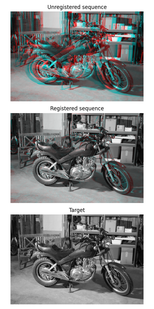
根据定义，光流是矢量场 (U，V) 验证 image1(x+u, y+v) = image0(x, y) ，其中(Image0，Image1)是来自序列的两个连续2D帧。然后，该向量场可用于通过图像扭曲进行配准。

为了显示配准结果，通过将配准结果分配给红色通道并且将目标图像分配给绿色和蓝色通道来构造RGB图像。完美配准会产生灰度级图像，而错误配准的像素在构建的RGB图像中显示为彩色。

import numpy as np
from matplotlib import pyplot as plt
from skimage.color import rgb2gray
from skimage.data import stereo_motorcycle, vortex
from skimage.transform import warp
from skimage.registration import optical_flow_tvl1, optical_flow_ilk

# --- Load the sequence
image0, image1, disp = stereo_motorcycle()

# --- Convert the images to gray level: color is not supported.
image0 = rgb2gray(image0)
image1 = rgb2gray(image1)

# --- Compute the optical flow
v, u = optical_flow_tvl1(image0, image1)

# --- Use the estimated optical flow for registration

nr, nc = image0.shape

row_coords, col_coords = np.meshgrid(np.arange(nr), np.arange(nc),
                                     indexing='ij')

image1_warp = warp(image1, np.array([row_coords + v, col_coords + u]),
                   mode='edge')

# build an RGB image with the unregistered sequence
seq_im = np.zeros((nr, nc, 3))
seq_im[..., 0] = image1
seq_im[..., 1] = image0
seq_im[..., 2] = image0

# build an RGB image with the registered sequence
reg_im = np.zeros((nr, nc, 3))
reg_im[..., 0] = image1_warp
reg_im[..., 1] = image0
reg_im[..., 2] = image0

# build an RGB image with the registered sequence
target_im = np.zeros((nr, nc, 3))
target_im[..., 0] = image0
target_im[..., 1] = image0
target_im[..., 2] = image0

# --- Show the result

fig, (ax0, ax1, ax2) = plt.subplots(3, 1, figsize=(5, 10))

ax0.imshow(seq_im)
ax0.set_title("Unregistered sequence")
ax0.set_axis_off()

ax1.imshow(reg_im)
ax1.set_title("Registered sequence")
ax1.set_axis_off()

ax2.imshow(target_im)
ax2.set_title("Target")
ax2.set_axis_off()

fig.tight_layout()

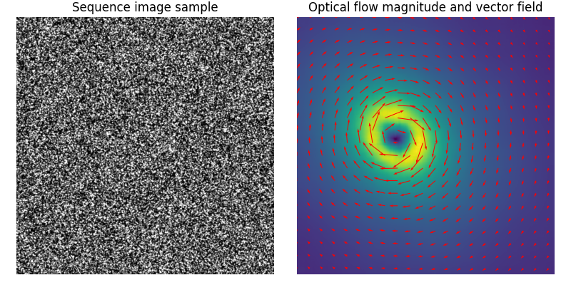
估计向量场 (U，V) 也可以用箭图显示。

在下面的例子中，迭代Lukas-Kanade算法(ILK)被应用于粒子图像测速(PIV)环境中的粒子图像。序列是案例B中的 PIV challenge 2001

image0, image1 = vortex()

# --- Compute the optical flow
v, u = optical_flow_ilk(image0, image1, radius=15)

# --- Compute flow magnitude
norm = np.sqrt(u ** 2 + v ** 2)

# --- Display
fig, (ax0, ax1) = plt.subplots(1, 2, figsize=(8, 4))

# --- Sequence image sample

ax0.imshow(image0, cmap='gray')
ax0.set_title("Sequence image sample")
ax0.set_axis_off()

# --- Quiver plot arguments

nvec = 20  # Number of vectors to be displayed along each image dimension
nl, nc = image0.shape
step = max(nl//nvec, nc//nvec)

y, x = np.mgrid[:nl:step, :nc:step]
u_ = u[::step, ::step]
v_ = v[::step, ::step]

ax1.imshow(norm)
ax1.quiver(x, y, u_, v_, color='r', units='dots',
           angles='xy', scale_units='xy', lw=3)
ax1.set_title("Optical flow magnitude and vector field")
ax1.set_axis_off()
fig.tight_layout()

plt.show()