滑动窗口直方图

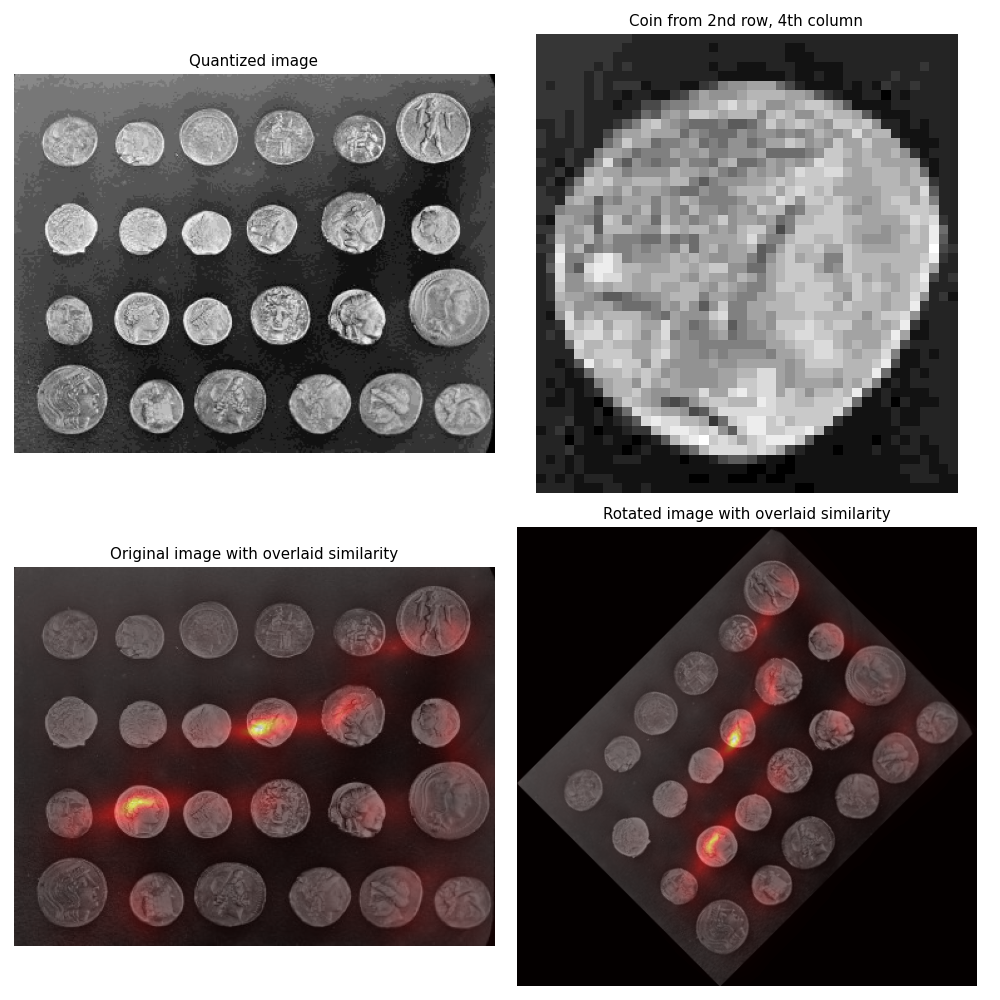
直方图匹配可用于图像中的目标检测 1. 此示例从 skimage.data.coins 图像，并使用直方图匹配尝试在原始图像中定位它。

首先，提取包含目标硬币的图像的盒状区域，并计算其灰度值的直方图。

接下来，对于测试图像中的每个像素，计算该像素周围的图像区域中的灰度值的直方图。 skimage.filters.rank.windowed_histogram 用于此任务，因为它使用了一种基于滑动窗口的高效算法，该算法能够快速计算这些直方图 2. 将图像中每个像素周围区域的局部直方图与单个硬币的局部直方图进行比较，并计算和显示相似性度量。

一枚硬币的直方图是用 numpy.histogram 而滑动窗口直方图是使用大小略有不同的圆盘状结构元素计算的。这样做是为了帮助证明，尽管存在这些差异，该技术仍然找到了相似之处。

为了证明该技术的旋转不变性，对旋转45度的硬币图像进行了相同的测试。

参考文献

1

Porikli、F.《积分直方图：在笛卡尔空间中快速提取直方图的方法》，CVPR，2005。IEEE，2005，第一卷

2

S.Perreault和P.Hebert。恒定时间中值滤波。翻译过来的。图像处理，16(9)：2389-2394,2007。

import numpy as np
import matplotlib
import matplotlib.pyplot as plt

from skimage import data, transform
from skimage.util import img_as_ubyte
from skimage.morphology import disk
from skimage.filters import rank


matplotlib.rcParams['font.size'] = 9


def windowed_histogram_similarity(image, selem, reference_hist, n_bins):
    # Compute normalized windowed histogram feature vector for each pixel
    px_histograms = rank.windowed_histogram(image, selem, n_bins=n_bins)

    # Reshape coin histogram to (1,1,N) for broadcast when we want to use it in
    # arithmetic operations with the windowed histograms from the image
    reference_hist = reference_hist.reshape((1, 1) + reference_hist.shape)

    # Compute Chi squared distance metric: sum((X-Y)^2 / (X+Y));
    # a measure of distance between histograms
    X = px_histograms
    Y = reference_hist

    num = (X - Y) ** 2
    denom = X + Y
    denom[denom == 0] = np.infty
    frac = num / denom

    chi_sqr = 0.5 * np.sum(frac, axis=2)

    # Generate a similarity measure. It needs to be low when distance is high
    # and high when distance is low; taking the reciprocal will do this.
    # Chi squared will always be >= 0, add small value to prevent divide by 0.
    similarity = 1 / (chi_sqr + 1.0e-4)

    return similarity


# Load the `skimage.data.coins` image
img = img_as_ubyte(data.coins())

# Quantize to 16 levels of greyscale; this way the output image will have a
# 16-dimensional feature vector per pixel
quantized_img = img // 16

# Select the coin from the 4th column, second row.
# Co-ordinate ordering: [x1,y1,x2,y2]
coin_coords = [184, 100, 228, 148]   # 44 x 44 region
coin = quantized_img[coin_coords[1]:coin_coords[3],
                     coin_coords[0]:coin_coords[2]]

# Compute coin histogram and normalize
coin_hist, _ = np.histogram(coin.flatten(), bins=16, range=(0, 16))
coin_hist = coin_hist.astype(float) / np.sum(coin_hist)

# Compute a disk shaped mask that will define the shape of our sliding window
# Example coin is ~44px across, so make a disk 61px wide (2 * rad + 1) to be
# big enough for other coins too.
selem = disk(30)

# Compute the similarity across the complete image
similarity = windowed_histogram_similarity(quantized_img, selem, coin_hist,
                                           coin_hist.shape[0])

# Now try a rotated image
rotated_img = img_as_ubyte(transform.rotate(img, 45.0, resize=True))
# Quantize to 16 levels as before
quantized_rotated_image = rotated_img // 16
# Similarity on rotated image
rotated_similarity = windowed_histogram_similarity(quantized_rotated_image,
                                                   selem, coin_hist,
                                                   coin_hist.shape[0])

fig, axes = plt.subplots(nrows=2, ncols=2, figsize=(10, 10))

axes[0, 0].imshow(quantized_img, cmap='gray')
axes[0, 0].set_title('Quantized image')
axes[0, 0].axis('off')

axes[0, 1].imshow(coin, cmap='gray')
axes[0, 1].set_title('Coin from 2nd row, 4th column')
axes[0, 1].axis('off')

axes[1, 0].imshow(img, cmap='gray')
axes[1, 0].imshow(similarity, cmap='hot', alpha=0.5)
axes[1, 0].set_title('Original image with overlaid similarity')
axes[1, 0].axis('off')

axes[1, 1].imshow(rotated_img, cmap='gray')
axes[1, 1].imshow(rotated_similarity, cmap='hot', alpha=0.5)
axes[1, 1].set_title('Rotated image with overlaid similarity')
axes[1, 1].axis('off')

plt.tight_layout()
plt.show()