形状指数

形状指数是局部曲率的单值度量，由Koenderink和van Doorn定义的黑森特征值得出 1.

它可以用来根据结构的外观局部形状来查找结构。

形状索引映射到从-1到1的值，表示不同类型的形状(有关详细信息，请参阅文档)。

在本例中，生成了一个带有斑点的随机图像，应该对其进行检测。

形状指数为1表示“球帽”，即我们要检测的斑点的形状。

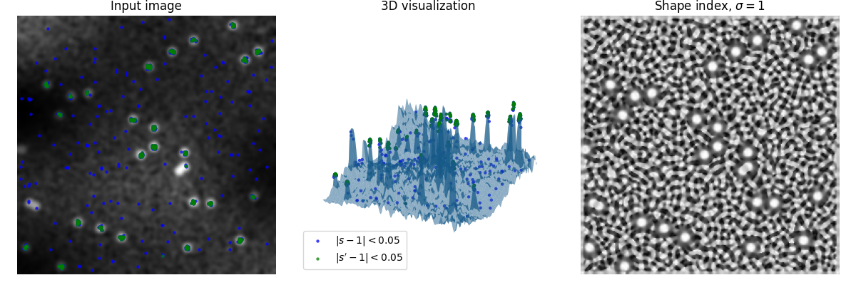
最左边的图显示生成的图像，中间的图显示图像的3D渲染，将强度值作为3D表面的高度，右边的图显示形状指数。

可见，形状指数也容易放大噪声的局部形状，但不受全局现象(例如，照明不均匀)的影响。

蓝色和绿色标记是与所需形状偏差不超过0.05的点。为了减弱信号中的噪声，在另一次高斯模糊传递(产生s‘)之后，从形状指数(S)中取出绿色标记。

注意相互连接得太近的点是如何 not 检测到，因为它们不具有所需的形状。

1

张晓明，“曲面形状与曲率尺度”，图像与视觉计算，1992，10,557-564。 DOI:10.1016/0262-8856(92)90076-F

import numpy as np
import matplotlib.pyplot as plt
from mpl_toolkits.mplot3d import Axes3D
from scipy import ndimage as ndi
from skimage.feature import shape_index
from skimage.draw import disk


def create_test_image(
        image_size=256, spot_count=30, spot_radius=5, cloud_noise_size=4):
    """
    Generate a test image with random noise, uneven illumination and spots.
    """
    state = np.random.get_state()
    np.random.seed(314159265)  # some digits of pi

    image = np.random.normal(
        loc=0.25,
        scale=0.25,
        size=(image_size, image_size)
    )

    for _ in range(spot_count):
        rr, cc = disk(
            (np.random.randint(image.shape[0]),
             np.random.randint(image.shape[1])),
            spot_radius,
            shape=image.shape
        )
        image[rr, cc] = 1

    image *= np.random.normal(loc=1.0, scale=0.1, size=image.shape)

    image *= ndi.zoom(
        np.random.normal(
            loc=1.0,
            scale=0.5,
            size=(cloud_noise_size, cloud_noise_size)
        ),
        image_size / cloud_noise_size
    )

    np.random.set_state(state)

    return ndi.gaussian_filter(image, sigma=2.0)

# First create the test image and its shape index

image = create_test_image()

s = shape_index(image)

# In this example we want to detect 'spherical caps',
# so we threshold the shape index map to
# find points which are 'spherical caps' (~1)

target = 1
delta = 0.05

point_y, point_x = np.where(np.abs(s - target) < delta)
point_z = image[point_y, point_x]

# The shape index map relentlessly produces the shape, even that of noise.
# In order to reduce the impact of noise, we apply a Gaussian filter to it,
# and show the results once in

s_smooth = ndi.gaussian_filter(s, sigma=0.5)

point_y_s, point_x_s = np.where(np.abs(s_smooth - target) < delta)
point_z_s = image[point_y_s, point_x_s]


fig = plt.figure(figsize=(12, 4))
ax1 = fig.add_subplot(1, 3, 1)

ax1.imshow(image, cmap=plt.cm.gray)
ax1.axis('off')
ax1.set_title('Input image')

scatter_settings = dict(alpha=0.75, s=10, linewidths=0)

ax1.scatter(point_x, point_y, color='blue', **scatter_settings)
ax1.scatter(point_x_s, point_y_s, color='green', **scatter_settings)

ax2 = fig.add_subplot(1, 3, 2, projection='3d', sharex=ax1, sharey=ax1)

x, y = np.meshgrid(
    np.arange(0, image.shape[0], 1),
    np.arange(0, image.shape[1], 1)
)

ax2.plot_surface(x, y, image, linewidth=0, alpha=0.5)

ax2.scatter(
    point_x,
    point_y,
    point_z,
    color='blue',
    label='$|s - 1|<0.05$',
    **scatter_settings
)

ax2.scatter(
    point_x_s,
    point_y_s,
    point_z_s,
    color='green',
    label='$|s\' - 1|<0.05$',
    **scatter_settings
)

ax2.legend(loc='lower left')

ax2.axis('off')
ax2.set_title('3D visualization')

ax3 = fig.add_subplot(1, 3, 3, sharex=ax1, sharey=ax1)

ax3.imshow(s, cmap=plt.cm.gray)
ax3.axis('off')
ax3.set_title(r'Shape index, $\sigma=1$')

fig.tight_layout()

plt.show()