用于纹理分类的局部二值模式

在这个例子中，我们将看到如何基于LBP(局部二进制模式)对纹理进行分类。LBP查看中心点周围的点，并测试周围的点是大于还是小于中心点(即给出一个二元结果)。

在图像上尝试LBP之前，查看LBPS的原理图会很有帮助。以下代码仅用于绘制原理图。

import numpy as np
import matplotlib.pyplot as plt


METHOD = 'uniform'
plt.rcParams['font.size'] = 9


def plot_circle(ax, center, radius, color):
    circle = plt.Circle(center, radius, facecolor=color, edgecolor='0.5')
    ax.add_patch(circle)


def plot_lbp_model(ax, binary_values):
    """Draw the schematic for a local binary pattern."""
    # Geometry spec
    theta = np.deg2rad(45)
    R = 1
    r = 0.15
    w = 1.5
    gray = '0.5'

    # Draw the central pixel.
    plot_circle(ax, (0, 0), radius=r, color=gray)
    # Draw the surrounding pixels.
    for i, facecolor in enumerate(binary_values):
        x = R * np.cos(i * theta)
        y = R * np.sin(i * theta)
        plot_circle(ax, (x, y), radius=r, color=str(facecolor))

    # Draw the pixel grid.
    for x in np.linspace(-w, w, 4):
        ax.axvline(x, color=gray)
        ax.axhline(x, color=gray)

    # Tweak the layout.
    ax.axis('image')
    ax.axis('off')
    size = w + 0.2
    ax.set_xlim(-size, size)
    ax.set_ylim(-size, size)


fig, axes = plt.subplots(ncols=5, figsize=(7, 2))

titles = ['flat', 'flat', 'edge', 'corner', 'non-uniform']

binary_patterns = [np.zeros(8),
                   np.ones(8),
                   np.hstack([np.ones(4), np.zeros(4)]),
                   np.hstack([np.zeros(3), np.ones(5)]),
                   [1, 0, 0, 1, 1, 1, 0, 0]]

for ax, values, name in zip(axes, binary_patterns, titles):
    plot_lbp_model(ax, values)
    ax.set_title(name)

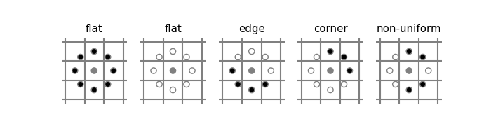
上图显示了使用黑色(或白色)表示的像素强度低于(或高于)中心像素的示例结果。当周围的像素全黑或全白时，该图像区域是平坦的(即无特征)。连续的黑色或白色像素组被认为是可以解释为角或边缘的“统一”图案。如果像素在黑白像素之间来回切换，则该图案被认为是“非均匀的”。

当使用LBP检测纹理时，您可以测量图像面片上的LBP集合，并查看这些LBP的分布。让我们将LBP应用于砖纹理。

from skimage.transform import rotate
from skimage.feature import local_binary_pattern
from skimage import data
from skimage.color import label2rgb

# settings for LBP
radius = 3
n_points = 8 * radius


def overlay_labels(image, lbp, labels):
    mask = np.logical_or.reduce([lbp == each for each in labels])
    return label2rgb(mask, image=image, bg_label=0, alpha=0.5)


def highlight_bars(bars, indexes):
    for i in indexes:
        bars[i].set_facecolor('r')


image = data.brick()
lbp = local_binary_pattern(image, n_points, radius, METHOD)


def hist(ax, lbp):
    n_bins = int(lbp.max() + 1)
    return ax.hist(lbp.ravel(), density=True, bins=n_bins, range=(0, n_bins),
                   facecolor='0.5')


# plot histograms of LBP of textures
fig, (ax_img, ax_hist) = plt.subplots(nrows=2, ncols=3, figsize=(9, 6))
plt.gray()

titles = ('edge', 'flat', 'corner')
w = width = radius - 1
edge_labels = range(n_points // 2 - w, n_points // 2 + w + 1)
flat_labels = list(range(0, w + 1)) + list(range(n_points - w, n_points + 2))
i_14 = n_points // 4            # 1/4th of the histogram
i_34 = 3 * (n_points // 4)      # 3/4th of the histogram
corner_labels = (list(range(i_14 - w, i_14 + w + 1)) +
                 list(range(i_34 - w, i_34 + w + 1)))

label_sets = (edge_labels, flat_labels, corner_labels)

for ax, labels in zip(ax_img, label_sets):
    ax.imshow(overlay_labels(image, lbp, labels))

for ax, labels, name in zip(ax_hist, label_sets, titles):
    counts, _, bars = hist(ax, lbp)
    highlight_bars(bars, labels)
    ax.set_ylim(top=np.max(counts[:-1]))
    ax.set_xlim(right=n_points + 2)
    ax.set_title(name)

ax_hist[0].set_ylabel('Percentage')
for ax in ax_img:
    ax.axis('off')

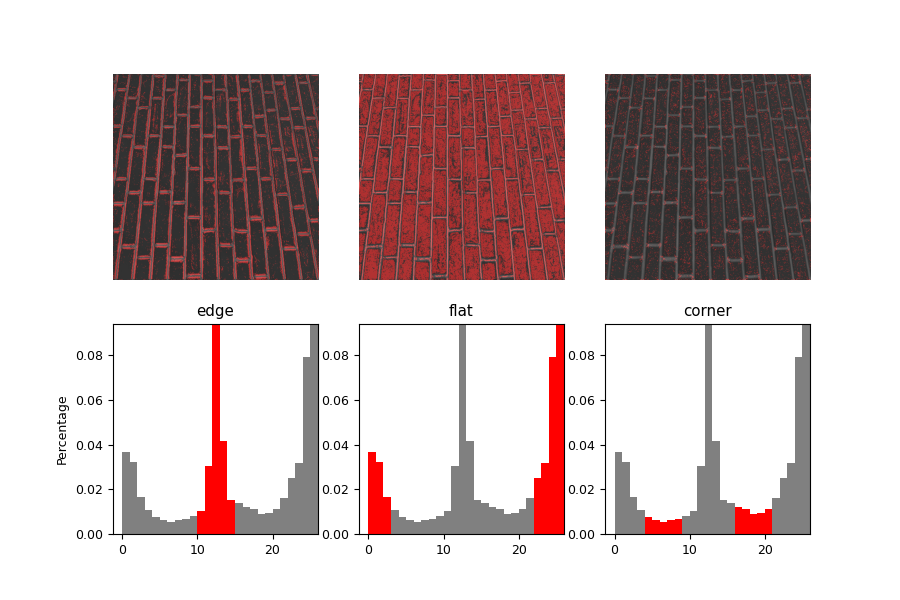
上图突出显示了图像的平坦、边状和角状区域。

LBP结果的直方图是一种很好的纹理分类方法。在这里，我们使用Kullback-Leibler散度来测试彼此之间的直方图分布。

# settings for LBP
radius = 2
n_points = 8 * radius


def kullback_leibler_divergence(p, q):
    p = np.asarray(p)
    q = np.asarray(q)
    filt = np.logical_and(p != 0, q != 0)
    return np.sum(p[filt] * np.log2(p[filt] / q[filt]))


def match(refs, img):
    best_score = 10
    best_name = None
    lbp = local_binary_pattern(img, n_points, radius, METHOD)
    n_bins = int(lbp.max() + 1)
    hist, _ = np.histogram(lbp, density=True, bins=n_bins, range=(0, n_bins))
    for name, ref in refs.items():
        ref_hist, _ = np.histogram(ref, density=True, bins=n_bins,
                                   range=(0, n_bins))
        score = kullback_leibler_divergence(hist, ref_hist)
        if score < best_score:
            best_score = score
            best_name = name
    return best_name


brick = data.brick()
grass = data.grass()
gravel = data.gravel()

refs = {
    'brick': local_binary_pattern(brick, n_points, radius, METHOD),
    'grass': local_binary_pattern(grass, n_points, radius, METHOD),
    'gravel': local_binary_pattern(gravel, n_points, radius, METHOD)
}

# classify rotated textures
print('Rotated images matched against references using LBP:')
print('original: brick, rotated: 30deg, match result: ',
      match(refs, rotate(brick, angle=30, resize=False)))
print('original: brick, rotated: 70deg, match result: ',
      match(refs, rotate(brick, angle=70, resize=False)))
print('original: grass, rotated: 145deg, match result: ',
      match(refs, rotate(grass, angle=145, resize=False)))

# plot histograms of LBP of textures
fig, ((ax1, ax2, ax3), (ax4, ax5, ax6)) = plt.subplots(nrows=2, ncols=3,
                                                       figsize=(9, 6))
plt.gray()

ax1.imshow(brick)
ax1.axis('off')
hist(ax4, refs['brick'])
ax4.set_ylabel('Percentage')

ax2.imshow(grass)
ax2.axis('off')
hist(ax5, refs['grass'])
ax5.set_xlabel('Uniform LBP values')

ax3.imshow(gravel)
ax3.axis('off')
hist(ax6, refs['gravel'])

plt.show()

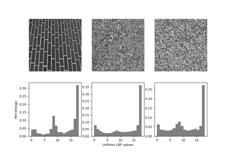
输出：

Rotated images matched against references using LBP:
original: brick, rotated: 30deg, match result:  brick
original: brick, rotated: 70deg, match result:  brick
original: grass, rotated: 145deg, match result:  grass