直线霍夫变换

霍夫变换最简单的形式是一种检测直线的方法 1.

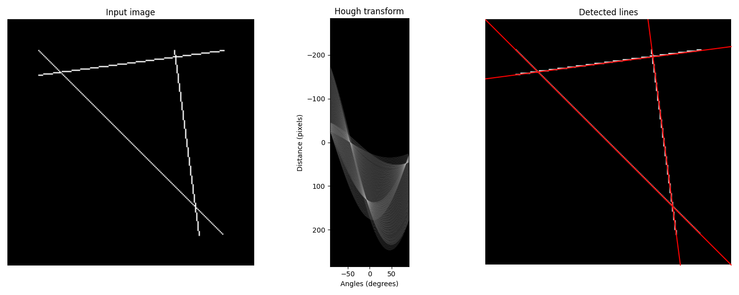
在下面的示例中，我们构建了一个具有直线交点的图像。然后，我们使用 Hough transform 。以探索可能贯穿图像的直线的参数空间。

算法概述

通常，线被参数化为 \(y = mx + c\) ，具有渐变 \(m\) 和Y-截取 c 。然而，这将意味着 \(m\) 对于垂直线来说是无穷大的。因此，我们将构建一条与该线垂直的线段，以指向原点。这条线由该线段的长度表示， \(r\) ，以及它与x轴的夹角， \(\theta\) 。

霍夫变换构造表示参数空间的直方图数组(即， \(M \times N\) 矩阵，用于 \(M\) 半径和半径的不同值 \(N\) 不同的价值观 \(\theta\) )。对于每个参数组合， \(r\) 和 \(\theta\) ，然后找出输入图像中接近相应行的非零像素数，并在位置处递增数组 \((r, \theta)\) 恰如其分。

我们可以想到每个非零像素为潜在的线条候选者“投票”。结果直方图中的局部最大值指示最可能线的参数。在我们的示例中，最大值出现在45度和135度，对应于每条线的法线向量角。

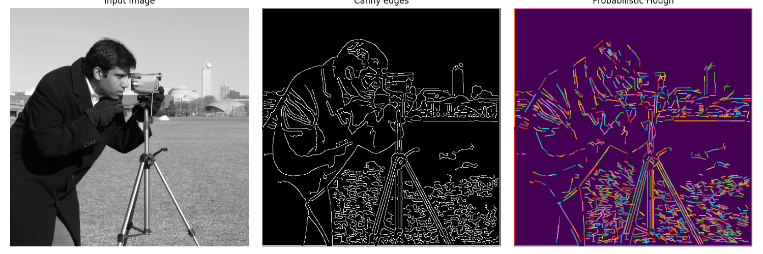
另一种方法是渐进概率Hough变换 2. 它基于这样的假设：使用随机的投票点子集可以很好地逼近实际结果，并且在投票过程中可以通过沿连通分量行走来提取直线。这将返回每个线段的开始和结束，这很有用。

该函数 probabilistic_hough 有三个参数：应用于霍夫累加器的一般阈值、最小线路长度和影响线路合并的线路间隙。在下面的示例中，我们发现长度大于10的行的间距小于3像素。

参考文献

1

杜达，R.O.和P.E.哈特，《使用霍夫变换来检测图像中的直线和曲线》，Comm。《美国医学杂志》，第15卷，第11-15页(1972年1月)

2

C.Galamhos，J.Matas和J.Kittler，《用于直线检测的渐进概率Hough变换》，IEEE计算机学会计算机视觉和模式识别会议，1999。

线霍夫变换

import numpy as np

from skimage.transform import hough_line, hough_line_peaks
from skimage.feature import canny
from skimage.draw import line
from skimage import data

import matplotlib.pyplot as plt
from matplotlib import cm


# Constructing test image
image = np.zeros((200, 200))
idx = np.arange(25, 175)
image[idx, idx] = 255
image[line(45, 25, 25, 175)] = 255
image[line(25, 135, 175, 155)] = 255

# Classic straight-line Hough transform
# Set a precision of 0.5 degree.
tested_angles = np.linspace(-np.pi / 2, np.pi / 2, 360, endpoint=False)
h, theta, d = hough_line(image, theta=tested_angles)

# Generating figure 1
fig, axes = plt.subplots(1, 3, figsize=(15, 6))
ax = axes.ravel()

ax[0].imshow(image, cmap=cm.gray)
ax[0].set_title('Input image')
ax[0].set_axis_off()

angle_step = 0.5 * np.diff(theta).mean()
d_step = 0.5 * np.diff(d).mean()
bounds = [np.rad2deg(theta[0] - angle_step),
          np.rad2deg(theta[-1] + angle_step),
          d[-1] + d_step, d[0] - d_step]
ax[1].imshow(np.log(1 + h), extent=bounds, cmap=cm.gray, aspect=1 / 1.5)
ax[1].set_title('Hough transform')
ax[1].set_xlabel('Angles (degrees)')
ax[1].set_ylabel('Distance (pixels)')
ax[1].axis('image')

ax[2].imshow(image, cmap=cm.gray)
origin = np.array((0, image.shape[1]))
for _, angle, dist in zip(*hough_line_peaks(h, theta, d)):
    y0, y1 = (dist - origin * np.cos(angle)) / np.sin(angle)
    ax[2].plot(origin, (y0, y1), '-r')
ax[2].set_xlim(origin)
ax[2].set_ylim((image.shape[0], 0))
ax[2].set_axis_off()
ax[2].set_title('Detected lines')

plt.tight_layout()
plt.show()

概率霍夫变换

from skimage.transform import probabilistic_hough_line

# Line finding using the Probabilistic Hough Transform
image = data.camera()
edges = canny(image, 2, 1, 25)
lines = probabilistic_hough_line(edges, threshold=10, line_length=5,
                                 line_gap=3)

# Generating figure 2
fig, axes = plt.subplots(1, 3, figsize=(15, 5), sharex=True, sharey=True)
ax = axes.ravel()

ax[0].imshow(image, cmap=cm.gray)
ax[0].set_title('Input image')

ax[1].imshow(edges, cmap=cm.gray)
ax[1].set_title('Canny edges')

ax[2].imshow(edges * 0)
for line in lines:
    p0, p1 = line
    ax[2].plot((p0[0], p1[0]), (p0[1], p1[1]))
ax[2].set_xlim((0, image.shape[1]))
ax[2].set_ylim((image.shape[0], 0))
ax[2].set_title('Probabilistic Hough')

for a in ax:
    a.set_axis_off()

plt.tight_layout()
plt.show()