圆形和椭圆形霍夫变换

霍夫变换最简单的形式是一个 method to detect straight lines 但它也可以用来检测圆形或椭圆形。该算法假设边缘被检测到，并且对噪声或缺失点具有健壮性。

圆检测

在下面的示例中，Hough变换用于检测硬币位置并匹配其边缘。我们提供了一系列合理的半径。对于每个半径，提取两个圆圈，最终保留五个最突出的候选对象。结果表明，该算法能够很好地检测硬币的位置。

算法概述

给出一个白色背景上的黑色圆圈，我们首先猜测它的半径(或半径范围)来构造一个新的圆圈。这个圆圈被应用于原始图片的每个黑色像素，并且这个圆圈的坐标在累加器中投票。从这种几何构造中，原始圆的中心位置获得最高分数。

请注意，累加器大小被构建为大于原始图片，以便检测帧外部的中心。它的大小是较大半径的两倍。

import numpy as np
import matplotlib.pyplot as plt

from skimage import data, color
from skimage.transform import hough_circle, hough_circle_peaks
from skimage.feature import canny
from skimage.draw import circle_perimeter
from skimage.util import img_as_ubyte


# Load picture and detect edges
image = img_as_ubyte(data.coins()[160:230, 70:270])
edges = canny(image, sigma=3, low_threshold=10, high_threshold=50)


# Detect two radii
hough_radii = np.arange(20, 35, 2)
hough_res = hough_circle(edges, hough_radii)

# Select the most prominent 3 circles
accums, cx, cy, radii = hough_circle_peaks(hough_res, hough_radii,
                                           total_num_peaks=3)

# Draw them
fig, ax = plt.subplots(ncols=1, nrows=1, figsize=(10, 4))
image = color.gray2rgb(image)
for center_y, center_x, radius in zip(cy, cx, radii):
    circy, circx = circle_perimeter(center_y, center_x, radius,
                                    shape=image.shape)
    image[circy, circx] = (220, 20, 20)

ax.imshow(image, cmap=plt.cm.gray)
plt.show()

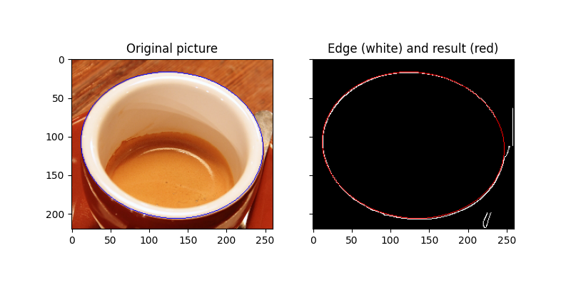
椭圆检测

在第二个示例中，目标是检测咖啡杯的边缘。基本上，这是一个圆的投影，即一个椭圆。要解决的问题要困难得多，因为必须确定五个参数，而不是圆的三个参数。

算法概述

该算法取属于椭圆的两个不同的点。它假定它是主轴。所有其他点上的循环决定了椭圆传递给这些点的量。良好的匹配对应于较高的累加器值。

该算法的完整描述可在参考文献中找到 1.

参考文献

1

谢永红和强记。“一种新的高效椭圆检测方法。”《模式识别》，2002。法律程序。第16届国际会议。第二卷，IEEE，2002

import matplotlib.pyplot as plt

from skimage import data, color, img_as_ubyte
from skimage.feature import canny
from skimage.transform import hough_ellipse
from skimage.draw import ellipse_perimeter

# Load picture, convert to grayscale and detect edges
image_rgb = data.coffee()[0:220, 160:420]
image_gray = color.rgb2gray(image_rgb)
edges = canny(image_gray, sigma=2.0,
              low_threshold=0.55, high_threshold=0.8)

# Perform a Hough Transform
# The accuracy corresponds to the bin size of a major axis.
# The value is chosen in order to get a single high accumulator.
# The threshold eliminates low accumulators
result = hough_ellipse(edges, accuracy=20, threshold=250,
                       min_size=100, max_size=120)
result.sort(order='accumulator')

# Estimated parameters for the ellipse
best = list(result[-1])
yc, xc, a, b = [int(round(x)) for x in best[1:5]]
orientation = best[5]

# Draw the ellipse on the original image
cy, cx = ellipse_perimeter(yc, xc, a, b, orientation)
image_rgb[cy, cx] = (0, 0, 255)
# Draw the edge (white) and the resulting ellipse (red)
edges = color.gray2rgb(img_as_ubyte(edges))
edges[cy, cx] = (250, 0, 0)

fig2, (ax1, ax2) = plt.subplots(ncols=2, nrows=1, figsize=(8, 4),
                                sharex=True, sharey=True)

ax1.set_title('Original picture')
ax1.imshow(image_rgb)

ax2.set_title('Edge (white) and result (red)')
ax2.imshow(edges)

plt.show()