LI阈值

1993年，Li和Lee提出了一种新的标准来寻找区分图像背景和前景的最佳阈值 1. 他们建议，尽量减少 cross-entropy 在大多数情况下，在前景和前景平均值之间，以及背景和背景平均值之间，将给出最佳阈值。

然而，直到1998年，找到这个阈值的方法是尝试所有可能的阈值，然后选择具有最小交叉熵的阈值。在这一点上，Li和Tam实现了一种新的迭代方法，通过使用交叉熵的斜率来更快地找到最优点 2. 这是在SCRKIT-IMAGE中实现的方法 skimage.filters.threshold_li() 。

在这里，我们用Li的迭代方法证明了交叉熵及其最优化。请注意，我们使用的是私有函数 _cross_entropy ，不应在生产代码中使用，因为它可能会更改。

1

李春华，李长康(1993)“最小交叉熵阈值”模式识别，26(4)：617-625 DOI:10.1016/0031-3203(93)90115-D

2

李春华，谭平山(1998)“最小交叉熵阈值的迭代算法”，模式识别通讯，18(8)：771-776 DOI:10.1016/S0167-8655(98)00057-9

import numpy as np
import matplotlib.pyplot as plt
from skimage import data
from skimage import filters
from skimage.filters.thresholding import _cross_entropy

cell = data.cell()
camera = data.camera()

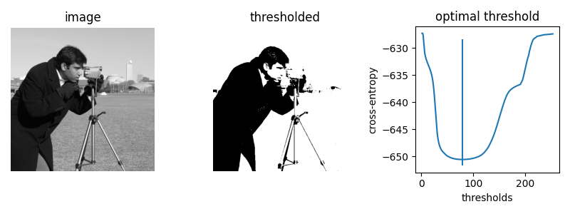
首先，让我们画出 skimage.data.camera() 在所有可能的阈值下成像。

thresholds = np.arange(np.min(camera) + 1.5, np.max(camera) - 1.5)
entropies = [_cross_entropy(camera, t) for t in thresholds]

optimal_camera_threshold = thresholds[np.argmin(entropies)]

fig, ax = plt.subplots(1, 3, figsize=(8, 3))

ax[0].imshow(camera, cmap='gray')
ax[0].set_title('image')
ax[0].set_axis_off()

ax[1].imshow(camera > optimal_camera_threshold, cmap='gray')
ax[1].set_title('thresholded')
ax[1].set_axis_off()

ax[2].plot(thresholds, entropies)
ax[2].set_xlabel('thresholds')
ax[2].set_ylabel('cross-entropy')
ax[2].vlines(optimal_camera_threshold,
             ymin=np.min(entropies) - 0.05 * np.ptp(entropies),
             ymax=np.max(entropies) - 0.05 * np.ptp(entropies))
ax[2].set_title('optimal threshold')

fig.tight_layout()

print('The brute force optimal threshold is:', optimal_camera_threshold)
print('The computed optimal threshold is:', filters.threshold_li(camera))

plt.show()

输出：

The brute force optimal threshold is: 78.5
The computed optimal threshold is: 78.91288426606151

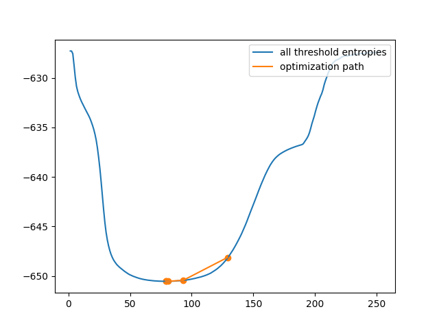
接下来，让我们使用 iter_callback 的特点 threshold_li 来检查发生时的优化过程。

iter_thresholds = []

optimal_threshold = filters.threshold_li(camera,
                                         iter_callback=iter_thresholds.append)
iter_entropies = [_cross_entropy(camera, t) for t in iter_thresholds]

print('Only', len(iter_thresholds), 'thresholds examined.')

fig, ax = plt.subplots()

ax.plot(thresholds, entropies, label='all threshold entropies')
ax.plot(iter_thresholds, iter_entropies, label='optimization path')
ax.scatter(iter_thresholds, iter_entropies, c='C1')
ax.legend(loc='upper right')

plt.show()

输出：

Only 5 thresholds examined.

这显然比暴力手段效率高得多。然而，在一些图像中，交叉熵不是 凸面 ，即只有一个最优解。在这种情况下，梯度下降可能会产生一个不是最优的阈值。在这个例子中，我们看到了对优化的糟糕的初始猜测如何导致糟糕的阈值选择。

iter_thresholds2 = []

opt_threshold2 = filters.threshold_li(cell, initial_guess=64,
                                      iter_callback=iter_thresholds2.append)

thresholds2 = np.arange(np.min(cell) + 1.5, np.max(cell) - 1.5)
entropies2 = [_cross_entropy(cell, t) for t in thresholds]
iter_entropies2 = [_cross_entropy(cell, t) for t in iter_thresholds2]

fig, ax = plt.subplots(1, 3, figsize=(8, 3))

ax[0].imshow(cell, cmap='magma')
ax[0].set_title('image')
ax[0].set_axis_off()

ax[1].imshow(cell > opt_threshold2, cmap='gray')
ax[1].set_title('thresholded')
ax[1].set_axis_off()

ax[2].plot(thresholds2, entropies2, label='all threshold entropies')
ax[2].plot(iter_thresholds2, iter_entropies2, label='optimization path')
ax[2].scatter(iter_thresholds2, iter_entropies2, c='C1')
ax[2].legend(loc='upper right')

plt.show()

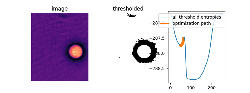
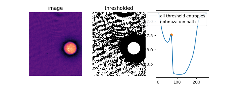
在这张图片中，令人惊讶的是， 默认设置 最初的猜测，即平均图像值，实际上是 正确的 在目标函数的两个“谷”之间的峰顶上。在不提供初始猜测的情况下，李的阈值方法根本不起作用！

iter_thresholds3 = []

opt_threshold3 = filters.threshold_li(cell,
                                      iter_callback=iter_thresholds3.append)

iter_entropies3 = [_cross_entropy(cell, t) for t in iter_thresholds3]

fig, ax = plt.subplots(1, 3, figsize=(8, 3))

ax[0].imshow(cell, cmap='magma')
ax[0].set_title('image')
ax[0].set_axis_off()

ax[1].imshow(cell > opt_threshold3, cmap='gray')
ax[1].set_title('thresholded')
ax[1].set_axis_off()

ax[2].plot(thresholds2, entropies2, label='all threshold entropies')
ax[2].plot(iter_thresholds3, iter_entropies3, label='optimization path')
ax[2].scatter(iter_thresholds3, iter_entropies3, c='C1')
ax[2].legend(loc='upper right')

plt.show()

为了了解情况，让我们定义一个函数， li_gradient ，它复制LI方法的内循环并返回 变化 从当前阈值到下一个阈值。当这个梯度为0时，我们处于所谓的 驻点 Li返回此值。当它是负值时，下一次门槛猜测会更低，当它是正数时，下一次猜测会更高。

在下面的图中，我们显示了当初始猜测在 正确的 在该熵峰值的一侧。我们覆盖阈值更新渐变，通过以下方式标记0渐变线和默认初始猜测 threshold_li 。

def li_gradient(image, t):
    """Find the threshold update at a given threshold."""
    foreground = image > t
    mean_fore = np.mean(image[foreground])
    mean_back = np.mean(image[~foreground])
    t_next = ((mean_back - mean_fore) /
              (np.log(mean_back) - np.log(mean_fore)))
    dt = t_next - t
    return dt


iter_thresholds4 = []
opt_threshold4 = filters.threshold_li(cell, initial_guess=68,
                                      iter_callback=iter_thresholds4.append)
iter_entropies4 = [_cross_entropy(cell, t) for t in iter_thresholds4]
print(len(iter_thresholds4), 'examined, optimum:', opt_threshold4)

gradients = [li_gradient(cell, t) for t in thresholds2]

fig, ax1 = plt.subplots()
ax1.plot(thresholds2, entropies2)
ax1.plot(iter_thresholds4, iter_entropies4)
ax1.scatter(iter_thresholds4, iter_entropies4, c='C1')
ax1.set_xlabel('threshold')
ax1.set_ylabel('cross entropy', color='C0')
ax1.tick_params(axis='y', labelcolor='C0')

ax2 = ax1.twinx()
ax2.plot(thresholds2, gradients, c='C3')
ax2.hlines([0], xmin=thresholds2[0], xmax=thresholds2[-1],
           colors='gray', linestyles='dashed')
ax2.vlines(np.mean(cell), ymin=np.min(gradients), ymax=np.max(gradients),
           colors='gray', linestyles='dashed')
ax2.set_ylabel(r'$\Delta$(threshold)', color='C3')
ax2.tick_params(axis='y', labelcolor='C3')

fig.tight_layout()

plt.show()

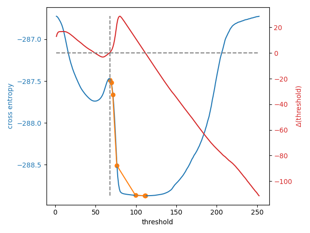
输出：

8 examined, optimum: 111.68876119648344

除了允许用户提供数字作为初始猜测之外， skimage.filters.threshold_li() 可以接收根据图像强度进行猜测的函数，就像 numpy.mean() 默认情况下为。当需要处理许多不同范围的图像时，这可能是一个很好的选择。

def quantile_95(image):
    # you can use np.quantile(image, 0.95) if you have NumPy>=1.15
    return np.percentile(image, 95)

iter_thresholds5 = []
opt_threshold5 = filters.threshold_li(cell, initial_guess=quantile_95,
                                      iter_callback=iter_thresholds5.append)
iter_entropies5 = [_cross_entropy(cell, t) for t in iter_thresholds5]
print(len(iter_thresholds5), 'examined, optimum:', opt_threshold5)

fig, ax1 = plt.subplots()
ax1.plot(thresholds2, entropies2)
ax1.plot(iter_thresholds5, iter_entropies5)
ax1.scatter(iter_thresholds5, iter_entropies5, c='C1')
ax1.set_xlabel('threshold')
ax1.set_ylabel('cross entropy', color='C0')
ax1.tick_params(axis='y', labelcolor='C0')

plt.show()

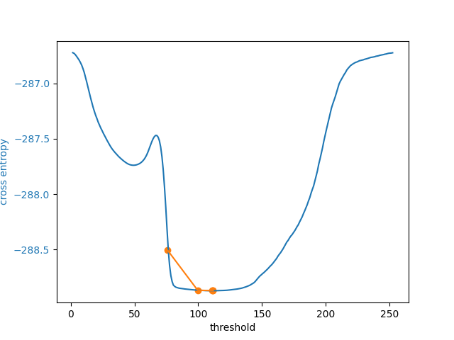
输出：

5 examined, optimum: 111.68876119648344