最大树

最大树是图像的分层表示，它是形态过滤器大家族的基础。

如果我们对一幅图像进行阈值运算，就会得到一个包含一个或多个连通分量的二值图像。如果我们应用较低的阈值，则来自较高阈值的所有连通分量都包含在来自较低阈值的连通分量中。这自然定义了可由树表示的嵌套组件的层次结构。当阈值T1的阈值得到的连通分量A包含在阈值T1<T2的阈值得到的分量B中时，我们说B是A的父树，所得到的树结构称为分量树。最大树是这种分量树的紧凑表示。 1, 2, 3, 4

在这个例子中，我们给出了一个最大树是什么的直觉。

参考文献

1

黄晓明(1998)。北京：北京：北京。用于图像和序列处理的反扩张连通算子。IEEE图像处理学报，7(4)，555-570。 DOI:10.1109/83.663500

2

伯杰，C.，Geraud，T.，Levillain，R.，Widynski，N.，Baillard，A.，Bertin，E.(2007)。有效分量树计算及其在天文成像模式识别中的应用载于国际图像处理会议(ICIP)(第41-44页)。 DOI:10.1109/ICIP.2007.4379949

3

Najman，L.，&Couprie，M.(2006)。在准线性时间内建立组件树。IEEE图像处理学报，15(11)，3531-3539。 DOI:10.1109/TIP.2006.877518

4

Carlinet，E.和Geraud，T.(2014)。组件树计算算法比较综述。IEEE图像处理学报，23(9)，3885-3895。 DOI:10.1109/TIP.2014.2336551

import numpy as np
import matplotlib.pyplot as plt
from matplotlib.lines import Line2D
from skimage.morphology import max_tree
import networkx as nx

在我们开始之前：几个助手函数

def plot_img(ax, image, title, plot_text, image_values):
    """Plot an image, overlaying image values or indices."""
    ax.imshow(image, cmap='gray', aspect='equal', vmin=0, vmax=np.max(image))
    ax.set_title(title)
    ax.set_yticks([])
    ax.set_xticks([])

    for x in np.arange(-0.5, image.shape[0], 1.0):
        ax.add_artist(Line2D((x, x), (-0.5, image.shape[0] - 0.5),
                             color='blue', linewidth=2))

    for y in np.arange(-0.5, image.shape[1], 1.0):
        ax.add_artist(Line2D((-0.5, image.shape[1]), (y, y),
                             color='blue', linewidth=2))

    if plot_text:
        for i, j in np.ndindex(*image_values.shape):
            ax.text(j, i, image_values[i, j], fontsize=8,
                    horizontalalignment='center',
                    verticalalignment='center',
                    color='red')
    return


def prune(G, node, res):
    """Transform a canonical max tree to a max tree."""
    value = G.nodes[node]['value']
    res[node] = str(node)
    preds = [p for p in G.predecessors(node)]
    for p in preds:
        if (G.nodes[p]['value'] == value):
            res[node] += ', %i' % p
            G.remove_node(p)
        else:
            prune(G, p, res)
    G.nodes[node]['label'] = res[node]
    return


def accumulate(G, node, res):
    """Transform a max tree to a component tree."""
    total = G.nodes[node]['label']
    parents = G.predecessors(node)
    for p in parents:
        total += ', ' + accumulate(G, p, res)
    res[node] = total
    return total


def position_nodes_for_max_tree(G, image_rav, root_x=4, delta_x=1.2):
    """Set the position of nodes of a max-tree.

    This function helps to visually distinguish between nodes at the same
    level of the hierarchy and nodes at different levels.
    """
    pos = {}
    for node in reversed(list(nx.topological_sort(canonical_max_tree))):
        value = G.nodes[node]['value']
        if canonical_max_tree.out_degree(node) == 0:
            # root
            pos[node] = (root_x, value)

        in_nodes = [y for y in canonical_max_tree.predecessors(node)]

        # place the nodes at the same level
        level_nodes = [y for y in
                       filter(lambda x: image_rav[x] == value, in_nodes)]
        nb_level_nodes = len(level_nodes) + 1

        c = nb_level_nodes // 2
        i = - c
        if (len(level_nodes) < 3):
            hy = 0
            m = 0
        else:
            hy = 0.25
            m = hy / (c - 1)

        for level_node in level_nodes:
            if(i == 0):
                i += 1
            if (len(level_nodes) < 3):
                pos[level_node] = (pos[node][0] + i * 0.6 * delta_x, value)
            else:
                pos[level_node] = (pos[node][0] + i * 0.6 * delta_x,
                                   value + m * (2 * np.abs(i) - c - 1))
            i += 1

        # place the nodes at different levels
        other_level_nodes = [y for y in
                             filter(lambda x: image_rav[x] > value, in_nodes)]
        if (len(other_level_nodes) == 1):
            i = 0
        else:
            i = - len(other_level_nodes) // 2
        for other_level_node in other_level_nodes:
            if((len(other_level_nodes) % 2 == 0) and (i == 0)):
                i += 1
            pos[other_level_node] = (pos[node][0] + i * delta_x,
                                     image_rav[other_level_node])
            i += 1

    return pos


def plot_tree(graph, positions, ax, *, title='', labels=None,
              font_size=8, text_size=8):
    """Plot max and component trees."""
    nx.draw_networkx(graph, pos=positions, ax=ax,
                     node_size=40, node_shape='s', node_color='white',
                     font_size=font_size, labels=labels)
    xlimit = ax.get_xlim()
    for v in range(image_rav.min(), image_rav.max() + 1):
        ax.hlines(v - 0.5, -3, 10, linestyles='dotted')
        ax.text(-3, v - 0.15, "val: %i" % v, fontsize=text_size)
    ax.hlines(v + 0.5, -3, 10, linestyles='dotted')
    ax.set_xlim(-3, 10)
    ax.set_title(title)
    ax.set_axis_off()

图像清晰度

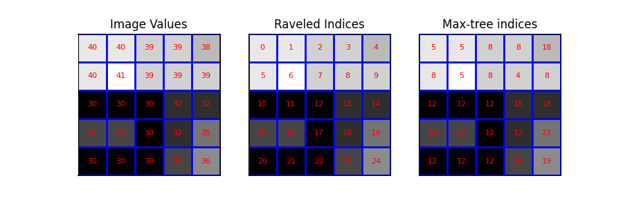
我们定义了一个小的测试图像。为了清晰起见，我们选择了一个示例图像，其中图像值不能与索引(不同范围)混淆。

image = np.array([[40, 40, 39, 39, 38],
                  [40, 41, 39, 39, 39],
                  [30, 30, 30, 32, 32],
                  [33, 33, 30, 32, 35],
                  [30, 30, 30, 33, 36]], dtype=np.uint8)

最大树

接下来，我们计算该图像的最大树。图像的最大树

P, S = max_tree(image)

P_rav = P.ravel()

图像地块

然后，我们将图像及其分解后的索引可视化。具体地说，我们使用以下覆盖来绘制图像：-图像值-分解的索引(用作像素标识符)-max_tree函数的输出

# raveled image
image_rav = image.ravel()

# raveled indices of the example image (for display purpose)
raveled_indices = np.arange(image.size).reshape(image.shape)

fig, (ax1, ax2, ax3) = plt.subplots(1, 3, sharey=True, figsize=(9, 3))

plot_img(ax1, image - image.min(), 'Image Values',
         plot_text=True, image_values=image)
plot_img(ax2, image - image.min(), 'Raveled Indices',
         plot_text=True, image_values=raveled_indices)
plot_img(ax3, image - image.min(), 'Max-tree indices',
         plot_text=True, image_values=P)

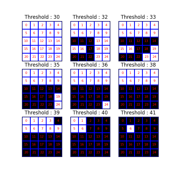
可视化阈值操作

现在，我们来研究一系列阈值运算的结果。组件树(和最大树)提供了不同级别的连接组件之间的包含关系的表示。

fig, axes = plt.subplots(3, 3, sharey=True, sharex=True, figsize=(6, 6))
thresholds = np.unique(image)
for k, threshold in enumerate(thresholds):
    bin_img = image >= threshold
    plot_img(axes[(k // 3), (k % 3)], bin_img, 'Threshold : %i' % threshold,
             plot_text=True, image_values=raveled_indices)

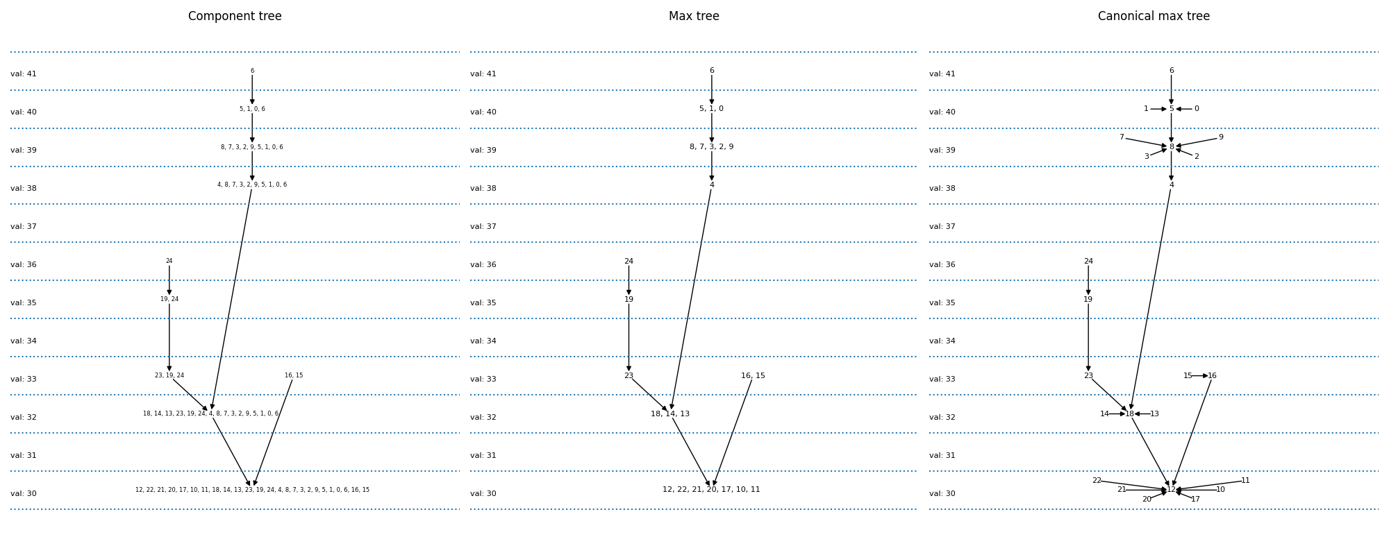
最大树图

现在，我们绘制分量和最大树。组件树将由所有可能的阈值操作产生的不同像素集彼此关联。如果一个级别的组件包含在较低级别的组件中，则图表中会有一个箭头。最大树只是像素集的一种不同编码。

1. 组件树：显式写出像素集。例如，我们看到{6}(在41处应用阈值的结果)是{0，1，5，6}(在40处的阈值)的父代。

2. 最大树：只有在该级别进入集合的像素才被显式写出。因此，我们将写入{6}->{0，1，5}而不是{6}->{0，1，5，6}

3. 规范的最大树L这是我们的实现所给出的表示。在这里，每个像素都是一个节点。几个像素的连通分量由其中一个像素表示。因此，我们将{6}->{0，1，5}替换为{6}->{5}，{1}->{5}，{0}->{5}，这允许我们通过图像(顶行，第三列)来表示图形。

# the canonical max-tree graph
canonical_max_tree = nx.DiGraph()
canonical_max_tree.add_nodes_from(S)
for node in canonical_max_tree.nodes():
    canonical_max_tree.nodes[node]['value'] = image_rav[node]
canonical_max_tree.add_edges_from([(n, P_rav[n]) for n in S[1:]])

# max-tree from the canonical max-tree
nx_max_tree = nx.DiGraph(canonical_max_tree)
labels = {}
prune(nx_max_tree, S[0], labels)

# component tree from the max-tree
labels_ct = {}
total = accumulate(nx_max_tree, S[0], labels_ct)

# positions of nodes : canonical max-tree (CMT)
pos_cmt = position_nodes_for_max_tree(canonical_max_tree, image_rav)

# positions of nodes : max-tree (MT)
pos_mt = dict(zip(nx_max_tree.nodes, [pos_cmt[node]
                                      for node in nx_max_tree.nodes]))

# plot the trees with networkx and matplotlib
fig, (ax1, ax2, ax3) = plt.subplots(1, 3, sharey=True, figsize=(20, 8))

plot_tree(nx_max_tree, pos_mt, ax1, title='Component tree',
          labels=labels_ct, font_size=6, text_size=8)

plot_tree(nx_max_tree, pos_mt, ax2, title='Max tree', labels=labels)

plot_tree(canonical_max_tree, pos_cmt, ax3, title='Canonical max tree')

fig.tight_layout()

plt.show()