对灰度图像进行着色

用某种颜色人为地给图像上色可能很有用，或者是为了突出图像的特定区域，或者只是为了使灰度图像生动起来。此示例通过缩放RGB值和调整HSV颜色空间中的颜色来演示图像着色。

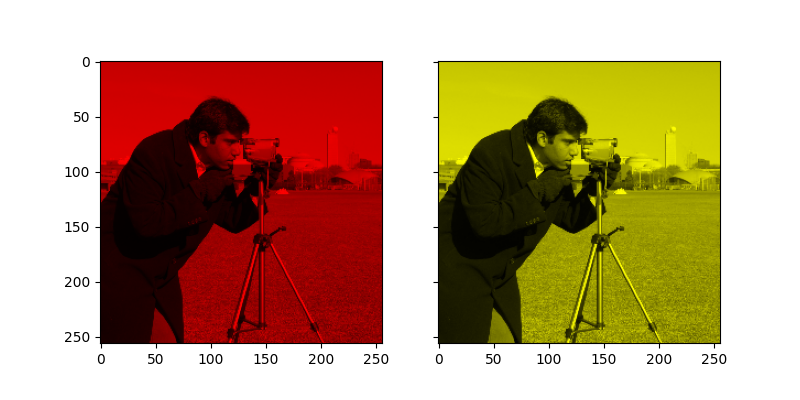
在2D中，彩色图像通常以RGB-3层2D阵列表示，其中这3层表示图像的(R)ED、(G)REEN和(B)LUE通道。获得彩色图像的最简单方法是将每个RGB通道设置为由每个通道的不同倍增缩放的灰度图像。例如，将绿色和蓝色通道乘以0将仅保留红色通道，并生成明亮的红色图像。同样，将蓝色通道调零只会留下红色和绿色通道，这两个通道组合在一起会形成黄色。

import matplotlib.pyplot as plt
from skimage import data
from skimage import color
from skimage import img_as_float

grayscale_image = img_as_float(data.camera()[::2, ::2])
image = color.gray2rgb(grayscale_image)

red_multiplier = [1, 0, 0]
yellow_multiplier = [1, 1, 0]

fig, (ax1, ax2) = plt.subplots(ncols=2, figsize=(8, 4),
                               sharex=True, sharey=True)
ax1.imshow(red_multiplier * image)
ax2.imshow(yellow_multiplier * image)

输出：

<matplotlib.image.AxesImage object at 0x7f2db106b6d0>

在许多情况下，处理RGB值可能并不理想。正因为如此，还有许多其他的 color spaces 其中您可以表示一幅彩色图像。一种流行的颜色空间称为HSV，它表示色调(~颜色)、饱和度(~彩色)和值(~亮度)。例如，一种颜色(色调)可能是绿色，但它的饱和度是绿色的强烈程度-橄榄色在低端，霓虹灯在高端。

在某些实现中，HSV中的色调从0到360，因为色调环绕在一个圆圈中。然而，在SCRKIT-IMAGE中，色调是从0到1的浮点值，因此色调、饱和度和值都共享相同的比例。

下面，我们在色调中绘制线性渐变，饱和度和值一直调高：

import numpy as np

hue_gradient = np.linspace(0, 1)
hsv = np.ones(shape=(1, len(hue_gradient), 3), dtype=float)
hsv[:, :, 0] = hue_gradient

all_hues = color.hsv2rgb(hsv)

fig, ax = plt.subplots(figsize=(5, 2))
# Set image extent so hues go from 0 to 1 and the image is a nice aspect ratio.
ax.imshow(all_hues, extent=(0 - 0.5 / len(hue_gradient),
                            1 + 0.5 / len(hue_gradient), 0, 0.2))
ax.set_axis_off()

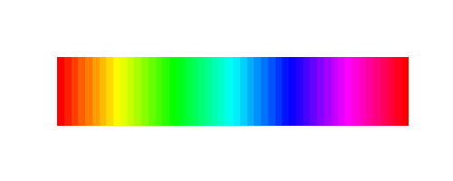
请注意最左侧和最右侧的颜色是如何相同的。这反映了这样一个事实，即色调像色轮一样环绕(请参见 HSV 了解更多信息)。

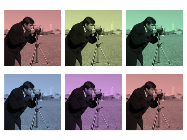
现在，让我们创建一个小实用函数来获取RGB图像并：

1.将RGB图像转换为HSV 2.设置色调和饱和度3.将HSV图像转换回RGB

def colorize(image, hue, saturation=1):
    """ Add color of the given hue to an RGB image.

    By default, set the saturation to 1 so that the colors pop!
    """
    hsv = color.rgb2hsv(image)
    hsv[:, :, 1] = saturation
    hsv[:, :, 0] = hue
    return color.hsv2rgb(hsv)

请注意，我们需要增加饱和度；饱和度为零的图像是灰度图像，因此我们需要一个非零值才能实际看到我们设置的颜色。

使用上面的函数，我们绘制了六幅具有色调线性渐变和非零饱和度的图像：

hue_rotations = np.linspace(0, 1, 6)

fig, axes = plt.subplots(nrows=2, ncols=3, sharex=True, sharey=True)

for ax, hue in zip(axes.flat, hue_rotations):
    # Turn down the saturation to give it that vintage look.
    tinted_image = colorize(image, hue, saturation=0.3)
    ax.imshow(tinted_image, vmin=0, vmax=1)
    ax.set_axis_off()
fig.tight_layout()

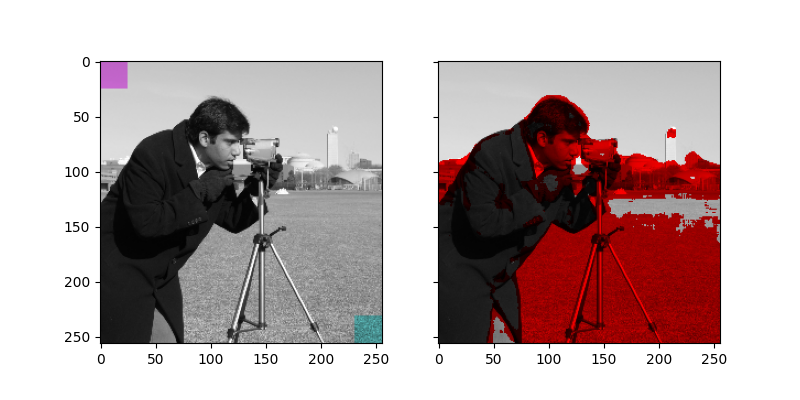
您可以将这种着色效果与麻木切片和花式索引相结合，以选择性地对图像进行着色。在下面的示例中，我们使用切片设置一些矩形的色调，并对通过阈值处理找到的一些像素的RGB值进行缩放。实际上，您可能希望根据分割结果或斑点检测方法定义着色区域。

from skimage.filters import rank

# Square regions defined as slices over the first two dimensions.
top_left = (slice(25),) * 2
bottom_right = (slice(-25, None),) * 2

sliced_image = image.copy()
sliced_image[top_left] = colorize(image[top_left], 0.82, saturation=0.5)
sliced_image[bottom_right] = colorize(image[bottom_right], 0.5, saturation=0.5)

# Create a mask selecting regions with interesting texture.
noisy = rank.entropy(grayscale_image, np.ones((9, 9)))
textured_regions = noisy > 4.25
# Note that using `colorize` here is a bit more difficult, since `rgb2hsv`
# expects an RGB image (height x width x channel), but fancy-indexing returns
# a set of RGB pixels (# pixels x channel).
masked_image = image.copy()
masked_image[textured_regions, :] *= red_multiplier

fig, (ax1, ax2) = plt.subplots(ncols=2, nrows=1, figsize=(8, 4),
                               sharex=True, sharey=True)
ax1.imshow(sliced_image)
ax2.imshow(masked_image)

plt.show()

输出：

/scikit-image/doc/examples/color_exposure/plot_tinting_grayscale_images.py:128: UserWarning:

Possible precision loss converting image of type float64 to uint8 as required by rank filters. Convert manually using skimage.util.img_as_ubyte to silence this warning.

对于为多个区域上色，您可能还会对 skimage.color.label2rgb 。