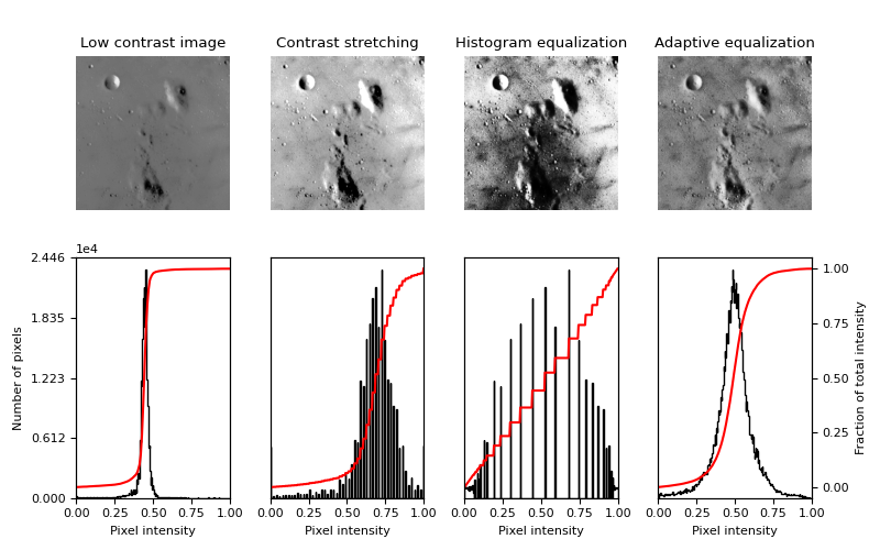
直方图均衡化

此示例使用一种名为 直方图均衡化 ，它在图像中“展开最频繁的强度值”。 1. 均衡后的图像具有大致线性的累积分布函数。

虽然直方图均衡化的优点是它不需要参数，但它有时会产生看起来不自然的图像。另一种方法是 对比度拉伸 ，其中图像被重新缩放以包括落在第二个和第98个百分位数内的所有亮度 2.

1

https://en.wikipedia.org/wiki/Histogram_equalization

2

http://homepages.inf.ed.ac.uk/rbf/HIPR2/stretch.htm

输出：

/scikit-image/doc/examples/color_exposure/plot_equalize.py:74: DeprecationWarning:

`np.object` is a deprecated alias for the builtin `object`. To silence this warning, use `object` by itself. Doing this will not modify any behavior and is safe.
Deprecated in NumPy 1.20; for more details and guidance: https://numpy.org/devdocs/release/1.20.0-notes.html#deprecations

import matplotlib
import matplotlib.pyplot as plt
import numpy as np

from skimage import data, img_as_float
from skimage import exposure


matplotlib.rcParams['font.size'] = 8


def plot_img_and_hist(image, axes, bins=256):
    """Plot an image along with its histogram and cumulative histogram.

    """
    image = img_as_float(image)
    ax_img, ax_hist = axes
    ax_cdf = ax_hist.twinx()

    # Display image
    ax_img.imshow(image, cmap=plt.cm.gray)
    ax_img.set_axis_off()

    # Display histogram
    ax_hist.hist(image.ravel(), bins=bins, histtype='step', color='black')
    ax_hist.ticklabel_format(axis='y', style='scientific', scilimits=(0, 0))
    ax_hist.set_xlabel('Pixel intensity')
    ax_hist.set_xlim(0, 1)
    ax_hist.set_yticks([])

    # Display cumulative distribution
    img_cdf, bins = exposure.cumulative_distribution(image, bins)
    ax_cdf.plot(bins, img_cdf, 'r')
    ax_cdf.set_yticks([])

    return ax_img, ax_hist, ax_cdf


# Load an example image
img = data.moon()

# Contrast stretching
p2, p98 = np.percentile(img, (2, 98))
img_rescale = exposure.rescale_intensity(img, in_range=(p2, p98))

# Equalization
img_eq = exposure.equalize_hist(img)

# Adaptive Equalization
img_adapteq = exposure.equalize_adapthist(img, clip_limit=0.03)

# Display results
fig = plt.figure(figsize=(8, 5))
axes = np.zeros((2, 4), dtype=np.object)
axes[0, 0] = fig.add_subplot(2, 4, 1)
for i in range(1, 4):
    axes[0, i] = fig.add_subplot(2, 4, 1+i, sharex=axes[0,0], sharey=axes[0,0])
for i in range(0, 4):
    axes[1, i] = fig.add_subplot(2, 4, 5+i)

ax_img, ax_hist, ax_cdf = plot_img_and_hist(img, axes[:, 0])
ax_img.set_title('Low contrast image')

y_min, y_max = ax_hist.get_ylim()
ax_hist.set_ylabel('Number of pixels')
ax_hist.set_yticks(np.linspace(0, y_max, 5))

ax_img, ax_hist, ax_cdf = plot_img_and_hist(img_rescale, axes[:, 1])
ax_img.set_title('Contrast stretching')

ax_img, ax_hist, ax_cdf = plot_img_and_hist(img_eq, axes[:, 2])
ax_img.set_title('Histogram equalization')

ax_img, ax_hist, ax_cdf = plot_img_and_hist(img_adapteq, axes[:, 3])
ax_img.set_title('Adaptive equalization')

ax_cdf.set_ylabel('Fraction of total intensity')
ax_cdf.set_yticks(np.linspace(0, 1, 5))

# prevent overlap of y-axis labels
fig.tight_layout()
plt.show()