阈值设置

阈值处理用于从灰度图像创建二值图像 1. 这是从背景中分割对象的最简单方法。

在SCRICKIT-IMAGE中实现的阈值算法可以分为两类：

• 基于直方图的。使用像素强度的直方图，并对该直方图的属性(例如，双峰)进行某些假设。

• 本地的。要处理像素，只使用相邻的像素。这些算法通常需要更多的计算时间。

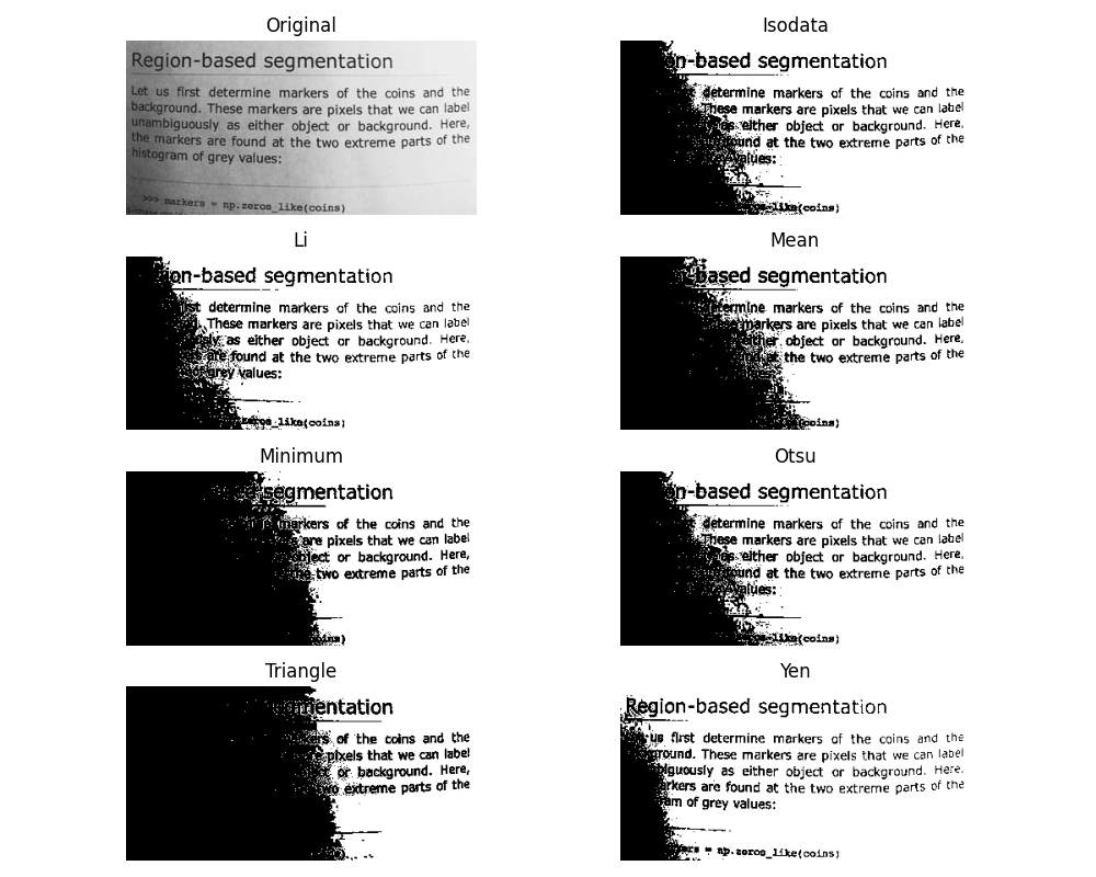
如果您不熟悉不同算法的细节和基本假设，通常很难知道哪种算法将提供最好的结果。因此，Scikit-Image包含了评价库提供的阈值算法的功能。一目了然，您可以为您的数据选择最好的算法，而无需深入了解它们的机制。

1

https://en.wikipedia.org/wiki/Thresholding_%28image_processing%29

参见

演示文稿 等级过滤器 。

import matplotlib.pyplot as plt

from skimage import data
from skimage.filters import try_all_threshold

img = data.page()

fig, ax = try_all_threshold(img, figsize=(10, 8), verbose=False)
plt.show()

如何设定门槛？

现在，我们将说明如何应用这些阈值算法之一。此示例使用像素强度的平均值。这是一个简单而幼稚的阈值，有时被用作猜测值。

from skimage.filters import threshold_mean


image = data.camera()
thresh = threshold_mean(image)
binary = image > thresh

fig, axes = plt.subplots(ncols=2, figsize=(8, 3))
ax = axes.ravel()

ax[0].imshow(image, cmap=plt.cm.gray)
ax[0].set_title('Original image')

ax[1].imshow(binary, cmap=plt.cm.gray)
ax[1].set_title('Result')

for a in ax:
    a.axis('off')

plt.show()

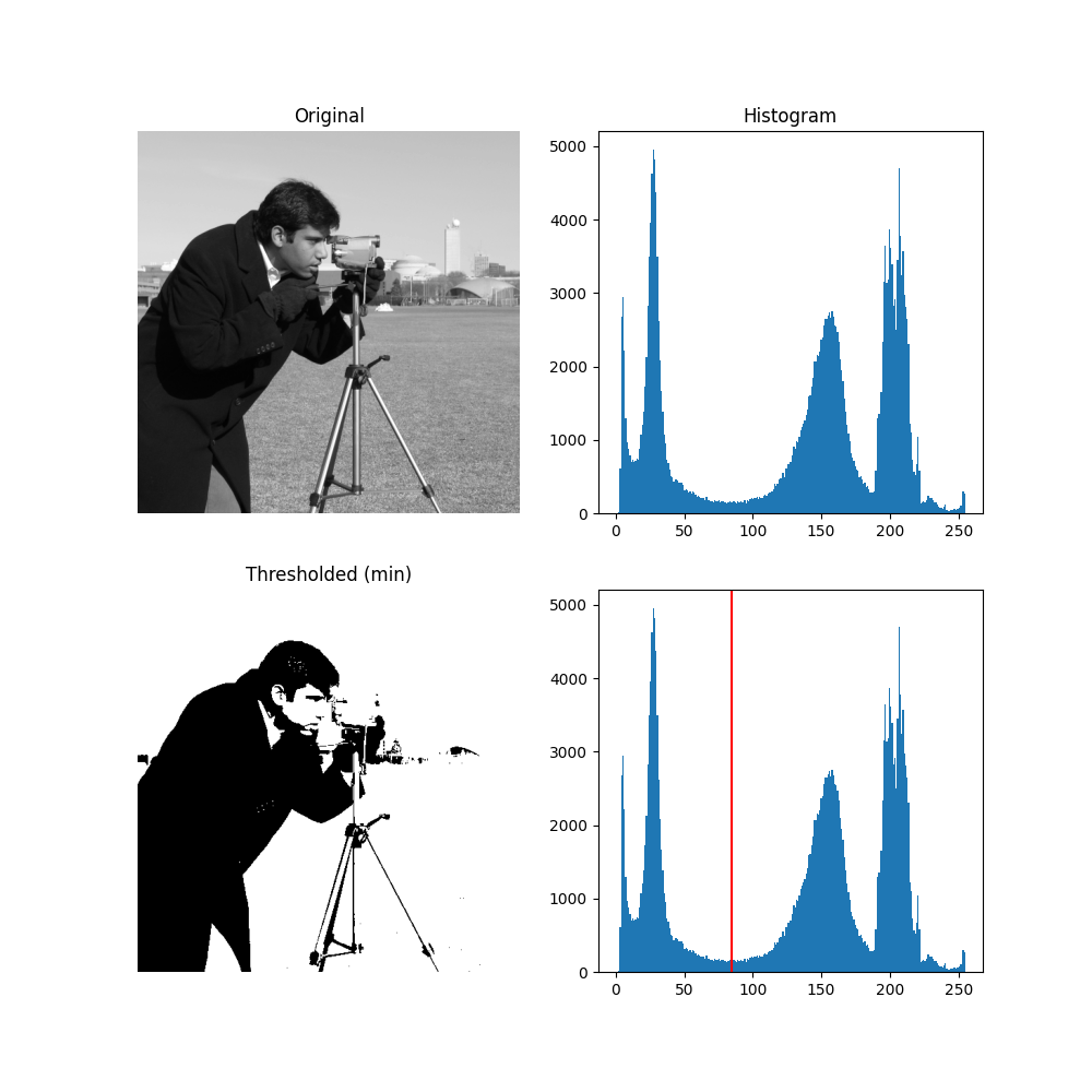
双峰直方图

对于具有双峰直方图的图片，可以使用更具体的算法。例如，最小值算法获取图像的直方图并反复对其进行平滑，直到直方图中只有两个峰值。

from skimage.filters import threshold_minimum


image = data.camera()

thresh_min = threshold_minimum(image)
binary_min = image > thresh_min

fig, ax = plt.subplots(2, 2, figsize=(10, 10))

ax[0, 0].imshow(image, cmap=plt.cm.gray)
ax[0, 0].set_title('Original')

ax[0, 1].hist(image.ravel(), bins=256)
ax[0, 1].set_title('Histogram')

ax[1, 0].imshow(binary_min, cmap=plt.cm.gray)
ax[1, 0].set_title('Thresholded (min)')

ax[1, 1].hist(image.ravel(), bins=256)
ax[1, 1].axvline(thresh_min, color='r')

for a in ax[:, 0]:
    a.axis('off')
plt.show()

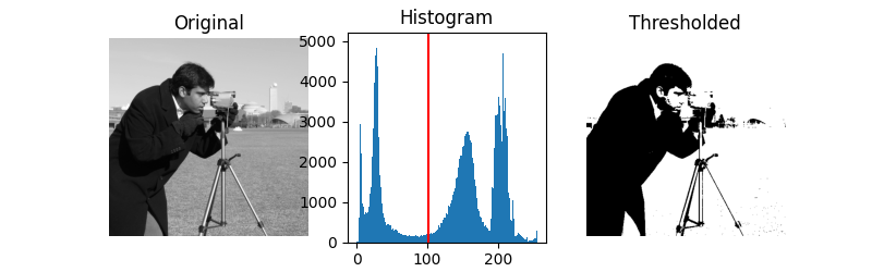
大津法 2 通过最大化由阈值分隔的两类像素之间的差异来计算“最佳”阈值(在下面的直方图中用红线标记)。等同地，该阈值最小化了类内方差。

2(1,2)

https://en.wikipedia.org/wiki/Otsu's_method

from skimage.filters import threshold_otsu


image = data.camera()
thresh = threshold_otsu(image)
binary = image > thresh

fig, axes = plt.subplots(ncols=3, figsize=(8, 2.5))
ax = axes.ravel()
ax[0] = plt.subplot(1, 3, 1)
ax[1] = plt.subplot(1, 3, 2)
ax[2] = plt.subplot(1, 3, 3, sharex=ax[0], sharey=ax[0])

ax[0].imshow(image, cmap=plt.cm.gray)
ax[0].set_title('Original')
ax[0].axis('off')

ax[1].hist(image.ravel(), bins=256)
ax[1].set_title('Histogram')
ax[1].axvline(thresh, color='r')

ax[2].imshow(binary, cmap=plt.cm.gray)
ax[2].set_title('Thresholded')
ax[2].axis('off')

plt.show()

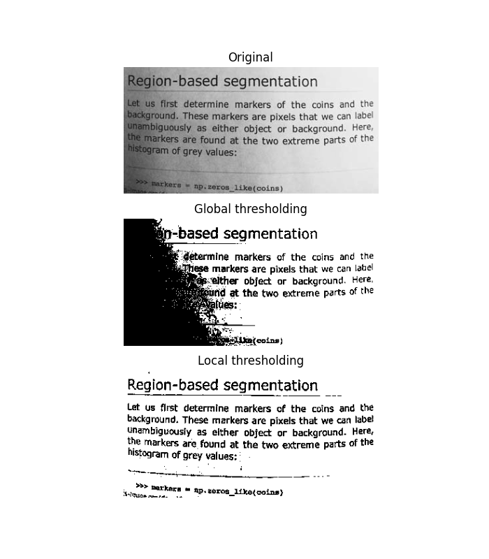
局部阈值

如果图像背景相对均匀，则可以使用如上所述的全局阈值。然而，如果背景强度有较大变化，则自适应阈值(也称为。局部或动态阈值)可能会产生更好的结果。请注意，局部阈值比全局阈值慢得多。

在这里，我们使用 threshold_local 函数，该函数计算具有特征大小的区域中的阈值 block_size 围绕每个像素(即本地邻居)。每个阈值是本地邻域减去偏移值的加权平均值。

from skimage.filters import threshold_otsu, threshold_local


image = data.page()

global_thresh = threshold_otsu(image)
binary_global = image > global_thresh

block_size = 35
local_thresh = threshold_local(image, block_size, offset=10)
binary_local = image > local_thresh

fig, axes = plt.subplots(nrows=3, figsize=(7, 8))
ax = axes.ravel()
plt.gray()

ax[0].imshow(image)
ax[0].set_title('Original')

ax[1].imshow(binary_global)
ax[1].set_title('Global thresholding')

ax[2].imshow(binary_local)
ax[2].set_title('Local thresholding')

for a in ax:
    a.axis('off')

plt.show()

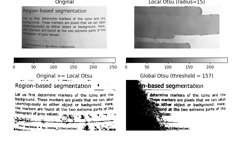
现在，我们来展示一下大津的门槛 2 方法可以在本地应用。对于每个像素，通过最大化由结构元素定义的局部邻域的两类像素之间的方差来确定最佳阈值。

该示例将本地阈值与全局阈值进行比较。

from skimage.morphology import disk
from skimage.filters import threshold_otsu, rank
from skimage.util import img_as_ubyte


img = img_as_ubyte(data.page())

radius = 15
selem = disk(radius)

local_otsu = rank.otsu(img, selem)
threshold_global_otsu = threshold_otsu(img)
global_otsu = img >= threshold_global_otsu

fig, axes = plt.subplots(2, 2, figsize=(8, 5), sharex=True, sharey=True)
ax = axes.ravel()
plt.tight_layout()

fig.colorbar(ax[0].imshow(img, cmap=plt.cm.gray),
             ax=ax[0], orientation='horizontal')
ax[0].set_title('Original')
ax[0].axis('off')

fig.colorbar(ax[1].imshow(local_otsu, cmap=plt.cm.gray),
             ax=ax[1], orientation='horizontal')
ax[1].set_title('Local Otsu (radius=%d)' % radius)
ax[1].axis('off')

ax[2].imshow(img >= local_otsu, cmap=plt.cm.gray)
ax[2].set_title('Original >= Local Otsu' % threshold_global_otsu)
ax[2].axis('off')

ax[3].imshow(global_otsu, cmap=plt.cm.gray)
ax[3].set_title('Global Otsu (threshold = %d)' % threshold_global_otsu)
ax[3].axis('off')

plt.show()