基于类Haar特征描述子的人脸分类

利用类Haar特征描述子实现了第一个实时人脸检测系统 1. 受这一应用的启发，我们提出了一个例子来说明如何提取、选择和分类类Haar特征来检测人脸和非人脸。

注意事项

此示例依赖于 scikit-learn 用于特征选择和分类。

参考文献

1

维奥拉、保罗和迈克尔·J·琼斯。“强大的实时人脸检测功能。”《国际计算机视觉杂志》57.2(2004)：137-154。Https://www.merl.com/publications/docs/TR2004-043.pdf DOI:10.1109/CVPR.2001.990517

import sys
from time import time

import numpy as np
import matplotlib.pyplot as plt

from dask import delayed

from sklearn.ensemble import RandomForestClassifier
from sklearn.model_selection import train_test_split
from sklearn.metrics import roc_auc_score

from skimage.data import lfw_subset
from skimage.transform import integral_image
from skimage.feature import haar_like_feature
from skimage.feature import haar_like_feature_coord
from skimage.feature import draw_haar_like_feature

从图像中提取类Haar特征的过程相对简单。首先定义了感兴趣区域(ROI)。其次，计算该感兴趣区域内的积分图像。最后，利用积分图像进行特征提取。

@delayed
def extract_feature_image(img, feature_type, feature_coord=None):
    """Extract the haar feature for the current image"""
    ii = integral_image(img)
    return haar_like_feature(ii, 0, 0, ii.shape[0], ii.shape[1],
                             feature_type=feature_type,
                             feature_coord=feature_coord)

我们使用了CBCL数据集的一个子集，它由100张人脸图像和100张非人脸图像组成。每幅图像的大小都调整为19x19像素的ROI。我们从每组图像中选择75幅图像来训练分类器，并确定最显著的特征。每类剩下的25幅图像被用来评估分类器的性能。

images = lfw_subset()
# To speed up the example, extract the two types of features only
feature_types = ['type-2-x', 'type-2-y']

# Build a computation graph using Dask. This allows the use of multiple
# CPU cores later during the actual computation
X = delayed(extract_feature_image(img, feature_types) for img in images)
# Compute the result
t_start = time()
X = np.array(X.compute(scheduler='threads'))
time_full_feature_comp = time() - t_start

# Label images (100 faces and 100 non-faces)
y = np.array([1] * 100 + [0] * 100)

X_train, X_test, y_train, y_test = train_test_split(X, y, train_size=150,
                                                    random_state=0,
                                                    stratify=y)

# Extract all possible features
feature_coord, feature_type = \
    haar_like_feature_coord(width=images.shape[2], height=images.shape[1],
                            feature_type=feature_types)

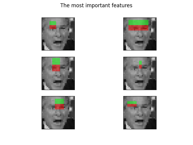
可以训练随机森林分类器以选择最显著的特征，特别是用于人脸分类。这个想法是为了确定树的整体最常使用的特征。通过在后续步骤中仅使用最显著的特征，我们可以在保持准确性的同时大幅加快计算速度。

# Train a random forest classifier and assess its performance
clf = RandomForestClassifier(n_estimators=1000, max_depth=None,
                             max_features=100, n_jobs=-1, random_state=0)
t_start = time()
clf.fit(X_train, y_train)
time_full_train = time() - t_start
auc_full_features = roc_auc_score(y_test, clf.predict_proba(X_test)[:, 1])

# Sort features in order of importance and plot the six most significant
idx_sorted = np.argsort(clf.feature_importances_)[::-1]

fig, axes = plt.subplots(3, 2)
for idx, ax in enumerate(axes.ravel()):
    image = images[0]
    image = draw_haar_like_feature(image, 0, 0,
                                   images.shape[2],
                                   images.shape[1],
                                   [feature_coord[idx_sorted[idx]]])
    ax.imshow(image)
    ax.set_xticks([])
    ax.set_yticks([])

_ = fig.suptitle('The most important features')

我们可以通过检查特征重要性的累积和来选择最重要的特征。在本例中，我们保留代表累积值的70%的特征(这对应于仅使用特征总数的3%)。

cdf_feature_importances = np.cumsum(clf.feature_importances_[idx_sorted])
cdf_feature_importances /= cdf_feature_importances[-1]  # divide by max value
sig_feature_count = np.count_nonzero(cdf_feature_importances < 0.7)
sig_feature_percent = round(sig_feature_count /
                            len(cdf_feature_importances) * 100, 1)
print(('{} features, or {}%, account for 70% of branch points in the '
       'random forest.').format(sig_feature_count, sig_feature_percent))

# Select the determined number of most informative features
feature_coord_sel = feature_coord[idx_sorted[:sig_feature_count]]
feature_type_sel = feature_type[idx_sorted[:sig_feature_count]]
# Note: it is also possible to select the features directly from the matrix X,
# but we would like to emphasize the usage of `feature_coord` and `feature_type`
# to recompute a subset of desired features.

# Build the computational graph using Dask
X = delayed(extract_feature_image(img, feature_type_sel, feature_coord_sel)
            for img in images)
# Compute the result
t_start = time()
X = np.array(X.compute(scheduler='threads'))
time_subs_feature_comp = time() - t_start

y = np.array([1] * 100 + [0] * 100)
X_train, X_test, y_train, y_test = train_test_split(X, y, train_size=150,
                                                    random_state=0,
                                                    stratify=y)

输出：

712 features, or 0.7%, account for 70% of branch points in the random forest.

一旦提取了特征，我们就可以训练和测试新的分类器。

t_start = time()
clf.fit(X_train, y_train)
time_subs_train = time() - t_start

auc_subs_features = roc_auc_score(y_test, clf.predict_proba(X_test)[:, 1])

summary = (('Computing the full feature set took {:.3f}s, plus {:.3f}s '
            'training, for an AUC of {:.2f}. Computing the restricted '
            'feature set took {:.3f}s, plus {:.3f}s training, '
            'for an AUC of {:.2f}.')
           .format(time_full_feature_comp, time_full_train,
                   auc_full_features, time_subs_feature_comp,
                   time_subs_train, auc_subs_features))

print(summary)
plt.show()

输出：

Computing the full feature set took 218.318s, plus 1.662s training, for an AUC of 1.00. Computing the restricted feature set took 0.212s, plus 1.475s training, for an AUC of 1.00.