基于边缘的分割和基于区域的分割比较

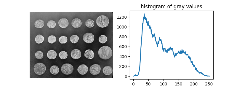
在这个例子中，我们将看到如何从背景中分割对象。我们使用 coins 图片来自 skimage.data ，它显示了几个硬币的轮廓在较暗的背景下。

import numpy as np
import matplotlib.pyplot as plt

from skimage import data
from skimage.exposure import histogram

coins = data.coins()
hist, hist_centers = histogram(coins)

fig, axes = plt.subplots(1, 2, figsize=(8, 3))
axes[0].imshow(coins, cmap=plt.cm.gray)
axes[0].axis('off')
axes[1].plot(hist_centers, hist, lw=2)
axes[1].set_title('histogram of gray values')

输出：

Text(0.5, 1.0, 'histogram of gray values')

阈值设置

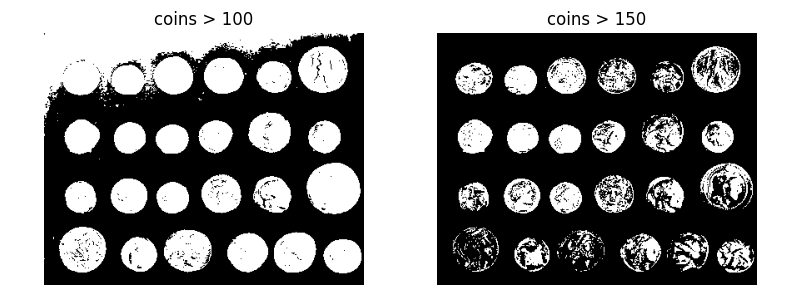
分割硬币的一种简单方法是根据灰度值的直方图选择阈值。不幸的是，对此图像进行阈值处理会得到一个二值图像，该图像要么遗漏了硬币的重要部分，要么将部分背景与硬币合并：

fig, axes = plt.subplots(1, 2, figsize=(8, 3), sharey=True)

axes[0].imshow(coins > 100, cmap=plt.cm.gray)
axes[0].set_title('coins > 100')

axes[1].imshow(coins > 150, cmap=plt.cm.gray)
axes[1].set_title('coins > 150')

for a in axes:
    a.axis('off')

plt.tight_layout()

基于边缘的分割

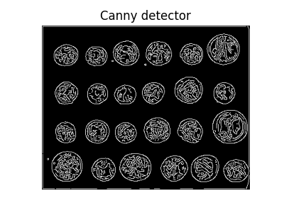
接下来，我们尝试使用基于边缘的分割来描绘硬币的轮廓。为了做到这一点，我们首先使用Canny边缘检测器获取特征的边缘。

from skimage.feature import canny

edges = canny(coins)

fig, ax = plt.subplots(figsize=(4, 3))
ax.imshow(edges, cmap=plt.cm.gray)
ax.set_title('Canny detector')
ax.axis('off')

输出：

(-0.5, 383.5, 302.5, -0.5)

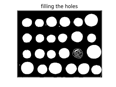
然后使用数学形态学填充这些轮廓。

from scipy import ndimage as ndi

fill_coins = ndi.binary_fill_holes(edges)

fig, ax = plt.subplots(figsize=(4, 3))
ax.imshow(fill_coins, cmap=plt.cm.gray)
ax.set_title('filling the holes')
ax.axis('off')

输出：

(-0.5, 383.5, 302.5, -0.5)

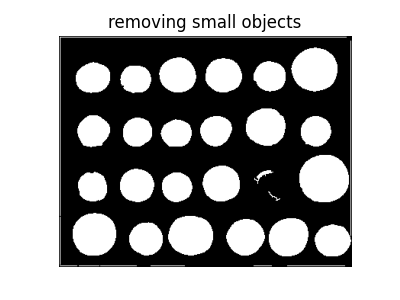
通过设置有效对象的最小大小，可以很容易地删除小的虚假对象。

from skimage import morphology

coins_cleaned = morphology.remove_small_objects(fill_coins, 21)

fig, ax = plt.subplots(figsize=(4, 3))
ax.imshow(coins_cleaned, cmap=plt.cm.gray)
ax.set_title('removing small objects')
ax.axis('off')

输出：

(-0.5, 383.5, 302.5, -0.5)

然而，这种方法不是很健壮，因为不是完全封闭的轮廓不能正确填充，就像上面一个未填充的硬币的情况一样。

基于区域的分割

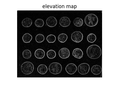
因此，我们尝试了一种使用分水岭变换的基于区域的方法。首先，我们使用图像的Sobel渐变找到一个高程地图。

from skimage.filters import sobel

elevation_map = sobel(coins)

fig, ax = plt.subplots(figsize=(4, 3))
ax.imshow(elevation_map, cmap=plt.cm.gray)
ax.set_title('elevation map')
ax.axis('off')

输出：

(-0.5, 383.5, 302.5, -0.5)

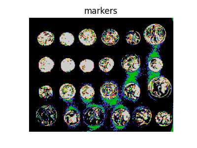
接下来，我们根据灰度值直方图的极端部分找到背景和硬币的标记。

markers = np.zeros_like(coins)
markers[coins < 30] = 1
markers[coins > 150] = 2

fig, ax = plt.subplots(figsize=(4, 3))
ax.imshow(markers, cmap=plt.cm.nipy_spectral)
ax.set_title('markers')
ax.axis('off')

输出：

(-0.5, 383.5, 302.5, -0.5)

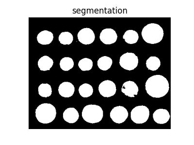
最后，我们使用分水岭变换从上面确定的标记开始填充立面地图的区域：

from skimage import segmentation

segmentation_coins = segmentation.watershed(elevation_map, markers)

fig, ax = plt.subplots(figsize=(4, 3))
ax.imshow(segmentation_coins, cmap=plt.cm.gray)
ax.set_title('segmentation')
ax.axis('off')

输出：

(-0.5, 383.5, 302.5, -0.5)

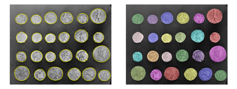
最后一种方法效果更好，硬币可以单独分割和标记。

from skimage.color import label2rgb

segmentation_coins = ndi.binary_fill_holes(segmentation_coins - 1)
labeled_coins, _ = ndi.label(segmentation_coins)
image_label_overlay = label2rgb(labeled_coins, image=coins, bg_label=0)

fig, axes = plt.subplots(1, 2, figsize=(8, 3), sharey=True)
axes[0].imshow(coins, cmap=plt.cm.gray)
axes[0].contour(segmentation_coins, [0.5], linewidths=1.2, colors='y')
axes[1].imshow(image_label_overlay)

for a in axes:
    a.axis('off')

plt.tight_layout()

plt.show()