注解
此笔记本可在此处下载: 02_CNN_1_Beauty.ipynb
MECA653学实干
从现有数据集创建简单的美容检测器
Hints: https://github.com/ustcqidi/BeautyPredict
问题陈述
我们将有一个网络摄像头输入。我们怎么才能算出美貌分数呢?
如何学习什么是美?
让我们使用卷积神经网络。
# Fix tensorflow without GPU :(  old cuda-10 but cuda-11.2 mismatch
# 1. Install miniconda
# 2. Install cuda-toolkit 11.2
# 3. Install cudnn 8.1
# 4. Install tensorflow-gpu

# !wget -nc https://repo.anaconda.com/miniconda/Miniconda3-latest-Linux-x86_64.sh
# !bash Miniconda3-latest-Linux-x86_64.sh -b -u
# !$HOME/miniconda3/bin/conda init bash
# !conda install cudatoolkit=11.2 -c conda-forge
# !conda install cudnn=8.1 -c conda-forge
# !python3 -m ipykernel install --user --name=base
# !$HOME/miniconda3/bin/pip3 install ipywidgets matplotlib pandas Pillow scipy tensorflow-gpu  # tf-nightly-gpu
from io import BytesIO
import urllib
from PIL import Image
import IPython
try:
    import ipywidgets as widgets
    from ipywidgets import interact, interact_manual
except ImportError:
    raise ImportError('ipywidgets is not installed.')

@interact
def predict_from_url(URL='https://upload.wikimedia.org/wikipedia/commons/c/c0/Nicolas_Cage_Deauville_2013.jpg'):
    with urllib.request.urlopen(URL) as url:  # Download an image from an URL in RAM memory
        img_size = 128
        img = Image.open(BytesIO(url.read())).convert('RGB')
        img = img.resize((img_size, img_size), Image.BILINEAR)
        IPython.display.display(img)  # Display the image

        # Preprocess image
        # img = tf.keras.preprocessing.image.img_to_array(img)
        # img = preprocess_input(img)
        # img = np.expand_dims(img, axis = 0)
        # prediction = model.predict(img)[0][0]  # Use da model
        # print('Predicted beauty:', prediction)
interactive(children=(Text(value='https://upload.wikimedia.org/wikipedia/commons/c/c0/Nicolas_Cage_Deauville_2…
1.创建数据集
%%capture
![ ! -d 'datasets' ] && echo 'datasets dir not found, will create' && mkdir datasets
![ ! -d 'logs' ] && echo 'logs dir not found, will create' && mkdir logs
![ ! -d 'models' ] && echo 'models dir not found, will create' && mkdir 'models'
![ ! -d './datasets/SCUT-FBP5500_v2' ] && echo './datasets/SCUT-FBP5500_v2 not found, will download & unzip it' && wget https://raw.githubusercontent.com/circulosmeos/gdown.pl/master/gdown.pl && perl gdown.pl 'https://drive.google.com/file/d/1w0TorBfTIqbquQVd6k3h_77ypnrvfGwf' './datasets/SCUT-FBP5500_v2.1.zip' && unzip -n -q -d './datasets/' './datasets/SCUT-FBP5500_v2.1.zip' && rm -f datasets/SCUT-FBP5500_v2.1.zip
我们现在将定义一些PATH变量来轻松访问数据集:
import os

dataset_path = os.path.relpath("datasets/SCUT-FBP5500_v2")
txt_file_path = os.path.join(dataset_path, "train_test_files", "All_labels.txt")
images_path = os.path.join(dataset_path, "Images")

assert os.path.exists(dataset_path)
assert os.path.exists(txt_file_path)
assert os.path.exists(images_path)

print("dataset_path:", dataset_path)
print("txt_file_path:", txt_file_path)
print("images_path:", images_path)
dataset_path: datasets/SCUT-FBP5500_v2
txt_file_path: datasets/SCUT-FBP5500_v2/train_test_files/All_labels.txt
images_path: datasets/SCUT-FBP5500_v2/Images
1.1浏览数据集
我们来看看里面有什么 ``datasets/SCUT-FBP5500_v2/train_test_files/All_labels.txt`` 。
txt_file_path 变量。import pandas as pd
# Mean rate by the 60th raters
df = "add your code to read the textfile in 'txt_file_path' with pandas"
# (columns should be names=["filename", "rating"] and the separator between columns should be a space))'
# WARNING: We will use the column names you just define next.
# By default it's set to "filename" and "rating".
# Next are some useful exploratory statistics:
# Check the 5th first row
# df.head()
# Describe the dataset
# df.describe()
# Rates histogram
# df.rating.hist(bins=30, density=1)
问题
平均评分是多少?
问题
评级范围是多少?
最低费率
最高速率
2.定义卷积神经网络
2.1.创建数据集加载器
为了训练一个神经网络,我们需要给它提供大量的图像作为输入。
import tensorflow as tf
import pkg_resources

for i, gpu in enumerate(tf.config.list_physical_devices('GPU')):
    print('Gpu %d:' % i, gpu)
print()

tf.config.experimental.set_memory_growth(tf.config.list_physical_devices('GPU')[0], True)

# Set mixed precision
if pkg_resources.parse_version(tf.__version__)  < pkg_resources.parse_version("2.4.0"):
    tf.keras.mixed_precision.experimental.set_policy("mixed_float16")
    print("Mixed precision policy:", tf.keras.mixed_precision.experimental.global_policy())
else:
    tf.keras.mixed_precision.set_global_policy("mixed_float16")
    print("Mixed precision policy:", tf.keras.mixed_precision.global_policy())
Gpu 0: PhysicalDevice(name='/physical_device:GPU:0', device_type='GPU')

INFO:tensorflow:Mixed precision compatibility check (mixed_float16): OK
Your GPU will likely run quickly with dtype policy mixed_float16 as it has compute capability of at least 7.0. Your GPU: GeForce RTX 3090, compute capability 8.6
Mixed precision policy: <Policy "mixed_float16">
import numpy as np
import time
from tensorflow.keras.applications.mobilenet_v2 import MobileNetV2, preprocess_input
# from tensorflow.keras.applications.mobilenet_v3 import MobileNetV3Small, preprocess_input
from tensorflow.keras.preprocessing.image import ImageDataGenerator


image_size = 128  # This low-resolution to increase speed
batch_size = 128  # This is the number of images per batches

validation_split = 0.2  # 0.2 -> 20% in validation, 80% in train
training_steps_per_epoch = (len(df) * (1 - validation_split)) // batch_size
validation_steps = (len(df) * validation_split) // batch_size


datagen = ImageDataGenerator(
    preprocessing_function=preprocess_input,  # This is what modify image color for ImageNet normalization
    validation_split=validation_split,
    fill_mode = 'nearest',
    # rotation_range=30,
    # width_shift_range=0.10,
    # height_shift_range=0.10,
    horizontal_flip=True,
    vertical_flip=False,
    # shear_range=0.05,  # Shear angle in counter-clockwise direction as radians.
    zoom_range=[0.7, 1.2],  # Float [1-value, 1+value] or [lower, upper] of random zoom.
    # brightness_range=[0.5, 1.8]  # Takes 100ms!  Random ratio [lower, upper] of brightness change.
)

train_generator = datagen.flow_from_dataframe(
    subset='training',
    dataframe=df,
    directory=images_path,
    x_col='filename', # name of col in data frame that contains file names
    y_col='rating',   # name of col with labels
    batch_size=batch_size,
    shuffle=True,
    target_size=(image_size, image_size),
    class_mode='raw',  # 'raw' is for regression, 'categorical' for classification task
)
validation_generator = datagen.flow_from_dataframe(
    subset='validation',
    dataframe=df,
    directory=images_path,
    x_col='filename', # name of col in data frame that contains file names
    y_col='rating',   # name of col with labels
    batch_size=batch_size,
    shuffle=True,
    target_size=(image_size, image_size),
    class_mode='raw'  # 'raw' is for regression, 'categorical' for classification task
)

train_dataset = tf.data.Dataset.from_generator(
    lambda: train_generator,
    output_types=(tf.float32, tf.float32),  # int32
    output_shapes=([None, image_size, image_size, 3], [None])  # None instead of a fixed batch_size for variable batch_size
)
validation_dataset = tf.data.Dataset.from_generator(
    lambda: train_generator,
    output_types=(tf.float32, tf.float32),
    output_shapes=([None, image_size, image_size, 3], [None])  # None instead of a fixed batch_size for variable batch_size
)
Found 4400 validated image filenames.
Found 1100 validated image filenames.
2.2-尝试并优化数据集加载器
现在,您可以通过计算一批图像来尝试数据集加载器。
import matplotlib.pyplot as plt


# Display the dataset
train_generator.image_data_generator.preprocessing_function=None  # Remove preprocessing
t1 = time.time()
x_batch, y_batch = next(train_generator)
print("Batch generation duration: %.2fs" % float(time.time()-t1))
train_generator.image_data_generator.preprocessing_function = preprocess_input  # Enable preprocessing

plt.figure(figsize=(12, 8), dpi=50)
plt.subplots_adjust(bottom=0, left=.01, right=1.2, top=0.9, hspace=0.2)
for i, (image, label) in enumerate(zip(x_batch[:32], y_batch[:32])):
    plt.subplot(4, 8, i + 1)
    plt.axis("off")
    plt.imshow(image.astype(np.uint8))
    plt.title("N°%i | Beauty: %.2f" % (i, label))
Batch generation duration: 0.39s

您可以看到图像已被修改:变形、亮度、对比度。
这就是所谓的 数据增强 。
问题
你能选择更好的增强参数吗?
2.3.定义神经网络
我们将使用 迁移学习 。
迁移学习意味着我们使用 pre-trained model ,但删除了预先培训的 last 图层。
我们添加自定义的最后一层 在上面 预先训练好的模型
然后我们只训练最后一个自定义图层
最后,我们可以对整个模型进行微调
选择好最后一层很重要 架构 。
你可以 hand-tune 此选项,或使用 AutoML (贝叶斯/遗传搜索)。
from tensorflow.keras.models import Sequential
from tensorflow.keras.layers import Activation, Dense, Dropout
from tensorflow.keras.optimizers import Adam


learning_rate = 0.001


def create_model():
    # Create a new neural networks model.
    model = Sequential(name='beautyNet')

    # Add a pre-trained model, without the last layer
    model.add(
        MobileNetV2(
            include_top=False,
            input_shape=(image_size, image_size, 3),
            pooling='avg',
            weights='imagenet')
    )

    # 1st layer as Dense with ReLu
    model.add(Dense(2, activation='relu'))

    # Add a stochastic regularization to avoid overfitting
    model.add(Dropout(rate=0.1))

    # Last layer as Dense for regression
    model.add(Dense(1, activation='linear'))

    # Do not train the first layer model, as it is already pre-trained
    model.layers[0].trainable = False

    # Compile the model with an optimizer
    model.compile(
        loss='mean_squared_error',  # 'mean_absolute_error', 'kullback_leibler_divergence'
        optimizer=Adam(learning_rate=learning_rate)
    )
    return model


model = create_model()
model.summary()
Model: "beautyNet"
_________________________________________________________________
Layer (type)                 Output Shape              Param #
=================================================================
mobilenetv2_1.00_128 (Functi (None, 1280)              2257984
_________________________________________________________________
dense (Dense)                (None, 8)                 10248
_________________________________________________________________
dropout (Dropout)            (None, 8)                 0
_________________________________________________________________
dense_1 (Dense)              (None, 1)                 9
=================================================================
Total params: 2,268,241
Trainable params: 10,257
Non-trainable params: 2,257,984
_________________________________________________________________
3.神经网络的训练
我们将使用 迁移学习 。
迁移学习意味着我们使用 pre-trained model ,但删除了预先培训的 last 图层。
我们添加自定义的最后一层 在上面 预先训练好的模型
然后我们只训练最后一个自定义图层
最后,我们可以对整个模型进行微调
选择好最后一层很重要 架构 。
你可以 hand-tune 模型体系结构和超参数,或使用 AutoML (贝叶斯/遗传搜索)。
import multiprocessing
from tensorflow.keras.callbacks import EarlyStopping, ModelCheckpoint, ReduceLROnPlateau


n_epochs = 20
initial_epoch = 0


callbacks = [
    EarlyStopping(
        monitor='val_loss',
        min_delta=1e-3,
        patience=10,
        verbose=1,
        ),
    ReduceLROnPlateau(
        monitor='val_loss',
        factor=0.2,
        patience=1,
        cooldown=1,
        min_lr=0.00001
        ),
    ModelCheckpoint(
        filepath='beauty_model_untuned_epoch{epoch:02d}.h5',
        monitor='val_loss',
        save_best_only=True,
        verbose=1
        )
]

t_start = time.time()
history = model.fit(
    train_dataset,
    epochs=n_epochs,
    callbacks=callbacks,
    initial_epoch=initial_epoch,
    steps_per_epoch=training_steps_per_epoch,
    validation_data=validation_dataset,
    validation_steps=validation_steps,
    workers=multiprocessing.cpu_count(),
)

print('Training duration: %.2fs' % float(time.time()-t_start))
Epoch 1/20
34/34 [==============================] - 35s 750ms/step - loss: 6.7363 - val_loss: 0.7023

Epoch 00001: val_loss improved from inf to 0.70233, saving model to beauty_model_untuned_epoch01.h5
Epoch 2/20
34/34 [==============================] - 17s 513ms/step - loss: 1.0485 - val_loss: 0.4525

Epoch 00002: val_loss improved from 0.70233 to 0.45248, saving model to beauty_model_untuned_epoch02.h5
Epoch 3/20
34/34 [==============================] - 17s 514ms/step - loss: 0.8943 - val_loss: 0.4391

Epoch 00003: val_loss improved from 0.45248 to 0.43915, saving model to beauty_model_untuned_epoch03.h5
Epoch 4/20
34/34 [==============================] - 17s 514ms/step - loss: 0.8333 - val_loss: 0.3691

Epoch 00004: val_loss improved from 0.43915 to 0.36914, saving model to beauty_model_untuned_epoch04.h5
Epoch 5/20
34/34 [==============================] - 17s 507ms/step - loss: 0.8411 - val_loss: 0.3352

Epoch 00005: val_loss improved from 0.36914 to 0.33523, saving model to beauty_model_untuned_epoch05.h5
Epoch 6/20
34/34 [==============================] - 17s 517ms/step - loss: 0.7894 - val_loss: 0.3365

Epoch 00006: val_loss did not improve from 0.33523
Epoch 7/20
34/34 [==============================] - 18s 518ms/step - loss: 0.7231 - val_loss: 0.3016

Epoch 00007: val_loss improved from 0.33523 to 0.30162, saving model to beauty_model_untuned_epoch07.h5
Epoch 8/20
34/34 [==============================] - 18s 520ms/step - loss: 0.8204 - val_loss: 0.3275

Epoch 00008: val_loss did not improve from 0.30162
Epoch 9/20
34/34 [==============================] - 18s 519ms/step - loss: 0.7342 - val_loss: 0.3100

Epoch 00009: val_loss did not improve from 0.30162
Epoch 10/20
34/34 [==============================] - 17s 509ms/step - loss: 0.7954 - val_loss: 0.3160

Epoch 00010: val_loss did not improve from 0.30162
Epoch 11/20
34/34 [==============================] - 17s 515ms/step - loss: 0.7924 - val_loss: 0.3228

Epoch 00011: val_loss did not improve from 0.30162
Epoch 12/20
34/34 [==============================] - 17s 514ms/step - loss: 0.7879 - val_loss: 0.2954

Epoch 00012: val_loss improved from 0.30162 to 0.29541, saving model to beauty_model_untuned_epoch12.h5
Epoch 13/20
34/34 [==============================] - 17s 513ms/step - loss: 0.8064 - val_loss: 0.3118

Epoch 00013: val_loss did not improve from 0.29541
Epoch 14/20
34/34 [==============================] - 17s 517ms/step - loss: 0.7649 - val_loss: 0.3405

Epoch 00014: val_loss did not improve from 0.29541
Epoch 15/20
34/34 [==============================] - 17s 507ms/step - loss: 0.7561 - val_loss: 0.3332

Epoch 00015: val_loss did not improve from 0.29541
Epoch 16/20
34/34 [==============================] - 17s 513ms/step - loss: 0.7468 - val_loss: 0.3339

Epoch 00016: val_loss did not improve from 0.29541
Epoch 17/20
34/34 [==============================] - 17s 517ms/step - loss: 0.7216 - val_loss: 0.3088

Epoch 00017: val_loss did not improve from 0.29541
Epoch 18/20
34/34 [==============================] - 17s 516ms/step - loss: 0.7925 - val_loss: 0.3528

Epoch 00018: val_loss did not improve from 0.29541
Epoch 19/20
34/34 [==============================] - 17s 516ms/step - loss: 0.7778 - val_loss: 0.3010

Epoch 00019: val_loss did not improve from 0.29541
Epoch 20/20
34/34 [==============================] - 17s 507ms/step - loss: 0.8443 - val_loss: 0.3242

Epoch 00020: val_loss did not improve from 0.29541
Training duration: 366.17s
# Evaluate (WARNING: you should use normaly unseen data)
test_loss = model.evaluate(train_generator, verbose=1)
print('Test loss: {:0.2f}'.format(test_loss))
35/35 [==============================] - 14s 396ms/step - loss: 0.2630
Test loss: 0.26
现在可以保存最终模型。
4.保存/加载训练好的模型
# Load a model from local checkpoints
epoch_id = 20

model_loaded = tf.keras.models.load_model('beauty_model_untuned_epoch%d.h5' % epoch_id)
# Save the final model
models_path = os.path.relpath("models")
assert os.path.exists(models_path)

# Save the final model
model.save(os.path.join(models_path, "beauty_model_untuned"))  # creates a HDF5 file 'final_beauty_model.h5'
INFO:tensorflow:Assets written to: models/beauty_model_untuned/assets
import os
import tensorflow as tf

# Load the final model
models_path = os.path.relpath("models")

model_loaded = tf.keras.models.load_model(os.path.join(models_path, "beauty_model_untuned"))
5.使用您的型号
# Predict on a new image
from io import BytesIO
import urllib
from PIL import Image
import IPython
import ipywidgets as widgets
from ipywidgets import interact, interact_manual


@interact
def predict_from_url(URL='https://upload.wikimedia.org/wikipedia/commons/c/c0/Nicolas_Cage_Deauville_2013.jpg'):
    with urllib.request.urlopen(URL) as url:  # Download an image from an URL in RAM memory
        img_size = 128
        img = Image.open(BytesIO(url.read())).convert('RGB')
        img = img.resize((img_size, img_size), Image.BILINEAR)

        # Preprocess image
        img_array = tf.keras.preprocessing.image.img_to_array(img)  # Convert PIL image to np.array
        img_batch = np.expand_dims(img_array, axis=0)  # Add a batch dim
        img_preprocessed = preprocess_input(img_batch)  # Normalize
        y_predicted = model.predict(img_preprocessed)  # Predict with your model

        IPython.display.display(img)  # Display the image
        print("Predicted beauty score:", y_predicted.flatten())
interactive(children=(Text(value='https://upload.wikimedia.org/wikipedia/commons/c/c0/Nicolas_Cage_Deauville_2…
6.在简单的Web应用程序中本地运行您的模型
我们可以使用Python包将Kera模型转换为TensorFlow.js格式 tensorflowjs 。
阅读有关以下内容的更多信息 converting Keras models to tfjs 。
live_demo 文件夹。!$HOME/miniconda3/bin/pip3 install -q tensorflowjs
import tensorflowjs as tfjs

tf.keras.backend.clear_session()  # Clean up variable names before exporting

# Convert model
model = tf.keras.models.load_model(os.path.join(models_path, "beauty_model_untuned"))
tfjs.converters.save_keras_model(model, "live_demo/model/",
                                 quantization_dtype_map={"uint8": "*"})

# Write an index.html file
with open('live_demo/index.html', 'w') as f:
  f.write('''
        <!DOCTYPE html>
        <html lang="en">
        <head>
          <meta charset="UTF-8" />
          <meta name="viewport" content="width=device-width, initial-scale=1.0" />
          <script src="https://cdn.jsdelivr.net/npm/@tensorflow/tfjs@latest"></script>
          <script src="https://cdn.jsdelivr.net/npm/@tensorflow-models/mobilenet"></script>
          <link rel="stylesheet" href="https://cdn.jsdelivr.net/npm/semantic-ui@2.4.2/dist/semantic.min.css" />
          <script src="https://cdn.jsdelivr.net/npm/semantic-ui@2.4.2/dist/semantic.min.js"></script>
          <style type="text/css">
            .app_container {
              width: 500px;
              display: flex;
              flex-direction: column;
              justify-content: center;
              align-items: center;}
            .ui .card {width: 90vw !important;}

            .content {
              display: flex;
              flex-direction: column;
            }

            .button_container {
              display: flex;
              flex-direction: row;
              justify-content: space-around;
              margin: 15px;
            }

            #output {
              font-size: 2em !important;
            }

            body {
              background-color: linen;
            }

            .stream {
              display: flex;
              overflow: hidden;
            }

            .card {
              min-width: 320px;
            }
          </style>

          <title>BeautyNet</title>
        </head>

        <body>
          <div class="ui one column centered grid" style="margin: 20px 0">
            <div class="app_container">
              <h1>BeautyNet</h1>
              <div class="ui card">
                <div class="stream">
                  <video width="100%" height="100%" autoplay playsinline muted id="webcam"></video>
                </div>
                <div class="content" id="content">
                  <div class="button_container">
                    <button class="ui primary button" id="capture">Save</button>
                    <button class="ui button" id="stop">Stop</button>
                  </div>
                  <div class="ui sub header" id="output"></div>
                </div>
              </div>
            </div>
          </div>
          <script>
            const modelPath = './model/model.json';
            const imageSize = 128;
            const predictionInterval = 500;
            var webcamElement = document.getElementById("webcam");
            var output = document.getElementById("output");
            var captureButton = document.getElementById("capture");
            var stopButton = document.getElementById("stop");
            var stopped = false;
            let model = null;

            async function setupWebcam() {
              return new Promise((resolve, reject) => {
                const navigatorAny = navigator;
                navigator.getUserMedia = navigator.getUserMedia ||
                  navigatorAny.webkitGetUserMedia || navigatorAny.mozGetUserMedia ||
                  navigatorAny.msGetUserMedia;
                if (navigator.getUserMedia) {
                  navigator.getUserMedia({
                      video: true
                    },
                    stream => {
                      webcamElement.srcObject = stream;
                      webcamElement.addEventListener("loadeddata", resolve, false);
                    },
                    error => reject());
                } else {
                  reject();
                }
              });
            }

            async function predictImage() {
              const img = await getWebcamImage();
              let result = tf.tidy(() => {
                const input = img.reshape([1, imageSize, imageSize, 3]);
                return model.predict(input);
              });
              img.dispose(); // Dispose the tensor to release the memory.
              let prediction = await result.data();
              result.dispose(); // Dispose the tensor to release the memory.
              output.innerText = `score: ${(prediction[0]).toFixed(1)}\n`;
            }

            async function getWebcamImage() {
              const img = (await webcam.capture()).toFloat();
              const normalized = img.div(127).sub(1);
              return normalized;
            }

            let webcam = null;
            let predictInterval;
            (async () => {
              // Load the model
              tf.loadLayersModel(modelPath)
                .then(response => {
                  model = response;
                  console.log("Model successfully loaded!");
                })
                .catch(error => output.textContent = "ERROR :" + error.message +
                  " Fix: put your model in a ./model/ folder")

              await setupWebcam();
              webcam = await tf.data.webcam(webcamElement, {
                resizeWidth: imageSize,
                resizeHeight: imageSize,
              });

              // Setup prediction every 500 ms
              predictInterval = setInterval(predictImage, predictionInterval);
            })();

            captureButton.addEventListener("click", async function () {
              const img = await getWebcamImage();
              let result = tf.tidy(() => {
                const input = img.reshape([1, imageSize, imageSize, 3]);
                return model.predict(input);
              });
              img.dispose(); // Dispose the tensor to release the memory.
              let prediction = await result.data();
              result.dispose(); // Dispose the tensor to release the memory.
              console.log("score", prediction[0]);
              output.innerText = `score: ${(prediction[0]).toFixed(1)}\n`;

              const div = document.createElement('div');
              div.innerText = `score: ${(prediction[0]).toFixed(3)}\n`;
              div.className = "description";
              document.getElementById("content").appendChild(div);
            });

            stopButton.addEventListener("click", function () {
              if (stopped == false) {
                clearInterval(predictInterval);

                stream = webcamElement.srcObject;
                tracks = stream.getTracks();
                tracks.forEach(function (track) {
                  track.stop();
                });
                stopButton.innerText = "Restart";
                stopped = true;
                console.log("Stop prediction");
              } else {
                (async () => {
                  await setupWebcam();
                  webcam = await tf.data.webcam(webcamElement, {
                    resizeWidth: imageSize,
                    resizeHeight: imageSize,
                  });
                  predictInterval = setInterval(predictImage, predictionInterval);
                  stopButton.innerText = "Stop";
                  stopped = false;
                  console.log("Prediction restarted");
                })();
              }
            });
          </script>
        </body>
        </html>
        ''')

!zip -r live_demo.zip live_demo

from IPython.display import FileLink
FileLink("live_demo.zip")
updating: live_demo/ (stored 0%)
updating: live_demo/index.html (deflated 63%)
updating: live_demo/model/ (stored 0%)
updating: live_demo/model/model.json (deflated 92%)
updating: live_demo/model/group1-shard1of1.bin (deflated 19%)
7.改善意见
!$HOME/miniconda3/bin/pip3 install -U tensorflow-addons
Requirement already up-to-date: tensorflow-addons in /usr/local/lib/python3.7/dist-packages (0.12.1)
Requirement already satisfied, skipping upgrade: typeguard>=2.7 in /usr/local/lib/python3.7/dist-packages (from tensorflow-addons) (2.7.1)
import datetime
import psutil
from tensorflow.keras.callbacks import EarlyStopping, ModelCheckpoint, TensorBoard
from tensorflow.keras.optimizers import Adam
import tensorflow_addons as tfa


# Cache dataset to RAM (WARNING: could OOM)
train_dataset = train_dataset.cache().prefetch(buffer_size=tf.data.experimental.AUTOTUNE)
validation_dataset = validation_dataset.cache().prefetch(buffer_size=tf.data.experimental.AUTOTUNE)


# Trace memory usage
class MemoryCallback(tf.keras.callbacks.Callback):
  def on_epoch_end(self, epoch, logs=None):
    bts = process.memory_info().rss  # in bytes
    # vbts = psutil.virtual_memory().used  # in bytes
    print(' RAM:', (bts / 1024) // 1024, 'MB')


process = psutil.Process(os.getpid())


# More epochs
n_epochs = 20


# Change learning rate over time
cyclic_rate_schelduler = tfa.optimizers.cyclical_learning_rate.Triangular2CyclicalLearningRate(
    initial_learning_rate=1e-4,
    maximal_learning_rate=0.005,
    # step_size=4 * training_steps_per_epoch,
    step_size=training_steps_per_epoch // 2,
    # scale_fn=lambda x: 1.,
    scale_mode='cycle',
    name='Triangular2CyclicalScheduler'
)

# Better optimizer
radam = tfa.optimizers.RectifiedAdam(learning_rate=cyclic_rate_schelduler)
ranger = tfa.optimizers.Lookahead(radam)

# Better loss
model.compile(optimizer=ranger, loss='mean_absolute_error')  # 'mean_absolute_percentage_error', 'mean_squared_error', 'kullback_leibler_divergence'
# Train with all these new things
t_start = time.time()
history = model.fit(
    train_dataset,
    epochs=n_epochs,
    callbacks=[*callbacks, MemoryCallback()],
    initial_epoch=initial_epoch,
    steps_per_epoch=training_steps_per_epoch,
    validation_data=validation_dataset,
    validation_steps=validation_steps,
    workers=multiprocessing.cpu_count(),
)

print("Training duration: %.2fs" % float(time.time()-t_start))
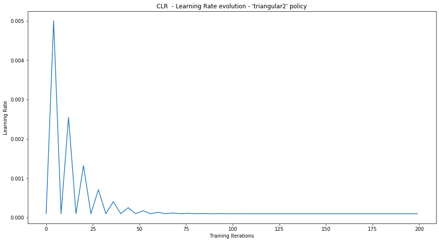
# View the learning rate evolution during training
plt.figure(1, figsize=(15, 8))
plt.xlabel("Training Iterations")
plt.ylabel("Learning Rate")
plt.title("CLR  - Learning Rate evolution - 'triangular2' policy")
plt.plot(range(0, n_epochs), [cyclic_rate_schelduler(i) for i in range(0, n_epochs)])
plt.show()
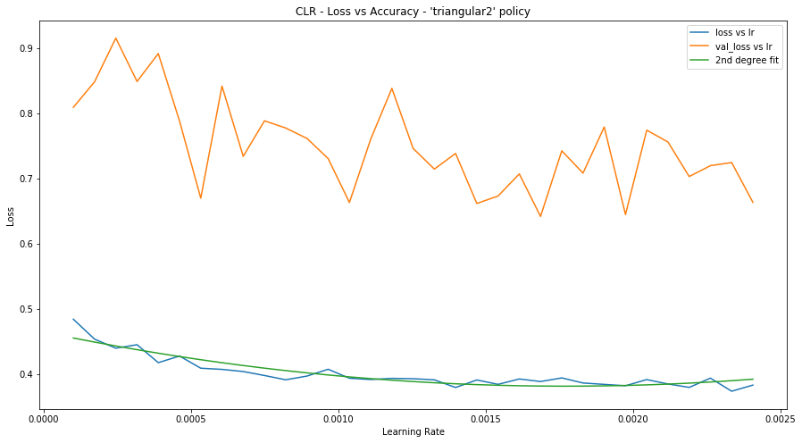
# View the learning rate evolution during training regarding the loss
plt.figure(1, figsize=(15, 8))
plt.xlabel("Learning Rate")
plt.ylabel("Loss")
plt.title("CLR - Loss vs Accuracy - 'triangular2' policy")
plt.plot([cyclic_rate_schelduler(i) for i in model.history.epoch], model.history.history["loss"])
plt.plot([cyclic_rate_schelduler(i) for i in model.history.epoch], model.history.history["val_loss"])

z = np.polyfit([cyclic_rate_schelduler(i) for i in model.history.epoch], model.history.history["loss"], 2)
p = np.poly1d(z)
plt.plot([cyclic_rate_schelduler(i) for i in model.history.epoch], p([cyclic_rate_schelduler(i) for i in model.history.epoch]))
plt.legend(["loss vs lr", "val_loss vs lr", "2nd degree fit"])

plt.show()
对数据加载器进行基准测试
# Benchmark your dataloader
import time


def benchmark(dataset, num_epochs=1, num_iter=100):
    start_time = time.perf_counter()
    for epoch_num in range(num_epochs):
        for iter_num, sample in enumerate(dataset):
            if iter_num > 100:
                print("break")
                break
            pass  # Performing a training step
    tf.print("Dataloader time per iter:", (time.perf_counter() - start_time) / (num_epochs * iter_num) )

benchmark(train_dataset)