注解
此笔记本可在此处下载: 1_ML_Tutorial_SVM.ipynb
1-支持向量机
from IPython.display import IFrame
IFrame('https://mljs.github.io/libsvm/#/SVC', width=800, height=800)
# Load the dataset
from keras.datasets import mnist
(x_train, y_train), (x_test, y_test) = mnist.load_data()
Using TensorFlow backend.
# Scale images from [0,255] to [0,1]
x_train_normalized = x_train / 255.0
import matplotlib
import matplotlib.pyplot as plt
%matplotlib inline
# %matplotlib nbagg
# %matplotlib ipympl
# %matplotlib notebook
import numpy as np
# Sample a smaller dataset for testing
rand_idx = np.random.choice(x_train.shape[0], 10000)
x_train = x_train_normalized[rand_idx]
y_train = y_train[rand_idx]
print('** What is the shape of your dataset? **')
(10000, 28, 28)
# Support Vector Machine
from sklearn import svm, metrics
# Create a Support Vector Classifier with the Defaults Scikit-Learn hyperparameters
clf = '** Add your code here **'
print('We have create an SVM Classifier with parameters:')
print(clf)
We have create an SVM Classifier with parameters:
SVC(C=1.0, cache_size=200, class_weight=None, coef0=0.0,
  decision_function_shape='ovr', degree=3, gamma=0.001, kernel='rbf',
  max_iter=-1, probability=False, random_state=None, shrinking=True,
  tol=0.001, verbose=False)
%time clf.fit(x_train.reshape(-1, 28 * 28), y_train)
CPU times: user 34.5 s, sys: 139 ms, total: 34.6 s
Wall time: 34.8 s
SVC(C=1.0, cache_size=200, class_weight=None, coef0=0.0,
  decision_function_shape='ovr', degree=3, gamma=0.001, kernel='rbf',
  max_iter=-1, probability=False, random_state=None, shrinking=True,
  tol=0.001, verbose=False)
# Validate the model performance: predict the classified digit from the test dataset
%time y_predicted = clf.predict(x_test.reshape(-1, 28 * 28))
CPU times: user 43.7 s, sys: 185 ms, total: 43.9 s
Wall time: 44.7 s
# What we should have predicted:
y_test
array([7, 2, 1, ..., 4, 5, 6], dtype=uint8)
# What we have predicted with our model:
y_predicted
array([2, 2, 2, ..., 2, 2, 2], dtype=uint8)
print("Classification report for classifier %s:\n%s\n" % (clf, metrics.classification_report(y_test, y_predicted)))
cm = metrics.confusion_matrix(y_test, y_predicted)
print("Confusion matrix:\n%s" % cm)

print("Accuracy={}".format(metrics.accuracy_score(y_test, y_predicted)))
Classification report for classifier SVC(C=1.0, cache_size=200, class_weight=None, coef0=0.0,
decision_function_shape='ovr', degree=3, gamma=0.001, kernel='rbf',
max_iter=-1, probability=False, random_state=None, shrinking=True,
tol=0.001, verbose=False):
precision recall f1-score support
0 0.00 0.00 0.00 980
1 0.00 0.00 0.00 1135
2 0.10 1.00 0.19 1032
3 0.00 0.00 0.00 1010
4 0.00 0.00 0.00 982
5 0.00 0.00 0.00 892
6 0.00 0.00 0.00 958
7 0.00 0.00 0.00 1028
8 0.00 0.00 0.00 974
9 0.00 0.00 0.00 1009
micro avg 0.10 0.10 0.10 10000
macro avg 0.01 0.10 0.02 10000
weighted avg 0.01 0.10 0.02 10000
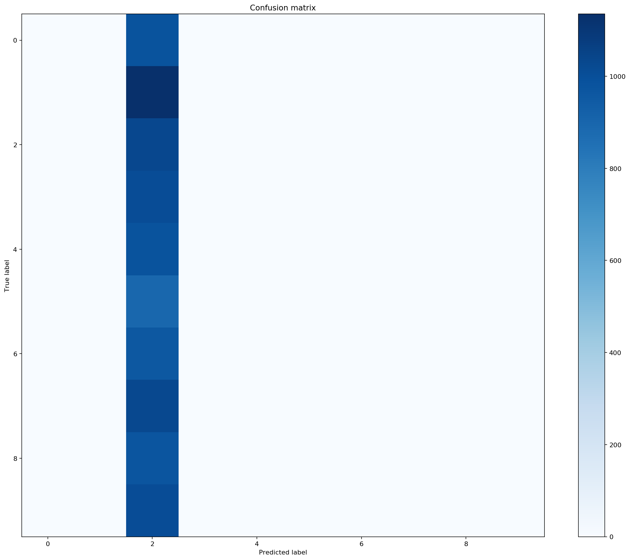
Confusion matrix:
[[ 0 0 980 0 0 0 0 0 0 0]
[ 0 0 1135 0 0 0 0 0 0 0]
[ 0 0 1032 0 0 0 0 0 0 0]
[ 0 0 1010 0 0 0 0 0 0 0]
[ 0 0 982 0 0 0 0 0 0 0]
[ 0 0 892 0 0 0 0 0 0 0]
[ 0 0 958 0 0 0 0 0 0 0]
[ 0 0 1028 0 0 0 0 0 0 0]
[ 0 0 974 0 0 0 0 0 0 0]
[ 0 0 1009 0 0 0 0 0 0 0]]
Accuracy=0.1032
/Users/Pierre/.virtualenvs/DeepQC/lib/python3.6/site-packages/sklearn/metrics/classification.py:1143: UndefinedMetricWarning: Precision and F-score are ill-defined and being set to 0.0 in labels with no predicted samples.
  'precision', 'predicted', average, warn_for)
#Plots confusion matrix
def plot_confusion_matrix(cm, title='Confusion matrix'):
    plt.figure(1, figsize=(15, 12), dpi=160)
    plt.imshow(cm, interpolation='nearest', cmap=plt.cm.Blues)
    plt.title(title)
    plt.colorbar()
    plt.tight_layout()
    plt.ylabel('True label')
    plt.xlabel('Predicted label')
    plt.show()

plot_confusion_matrix(cm)
2-超参数调整:更好更快地分类
# Hyperparameters tuning: better and faster
clf_faster = '** Add your code here **'  # Faster with linear kernel + handtuned C and gamma
print('We have create a faster SVM Classifier with parameters:')
print(clf_faster)
We have create a faster SVM Classifier with parameters:
SVC(C=5, cache_size=200, class_weight=None, coef0=0.0,
  decision_function_shape='ovr', degree=3, gamma=0.05, kernel='linear',
  max_iter=-1, probability=False, random_state=None, shrinking=True,
  tol=0.001, verbose=False)
%time clf_faster.fit(x_train.reshape(-1, 28 * 28), y_train)
CPU times: user 12.1 s, sys: 58.9 ms, total: 12.2 s
Wall time: 12.5 s
SVC(C=5, cache_size=200, class_weight=None, coef0=0.0,
  decision_function_shape='ovr', degree=3, gamma=0.05, kernel='linear',
  max_iter=-1, probability=False, random_state=None, shrinking=True,
  tol=0.001, verbose=False)
# Validate the model performance: predict the classified digit from the test dataset
%time y_predicted = clf_faster.predict(x_test.reshape(-1, 28 * 28))
y_predicted
CPU times: user 20.1 s, sys: 81.2 ms, total: 20.2 s
Wall time: 20.8 s
array([3, 2, 1, ..., 4, 8, 6], dtype=uint8)
print("Classification report for classifier %s:\n%s\n" % (clf_faster, metrics.classification_report(y_test, y_predicted)))
cm = metrics.confusion_matrix(y_test, y_predicted)
print("Confusion matrix:\n%s" % cm)
print("Accuracy={}".format(metrics.accuracy_score(y_test, y_predicted)))
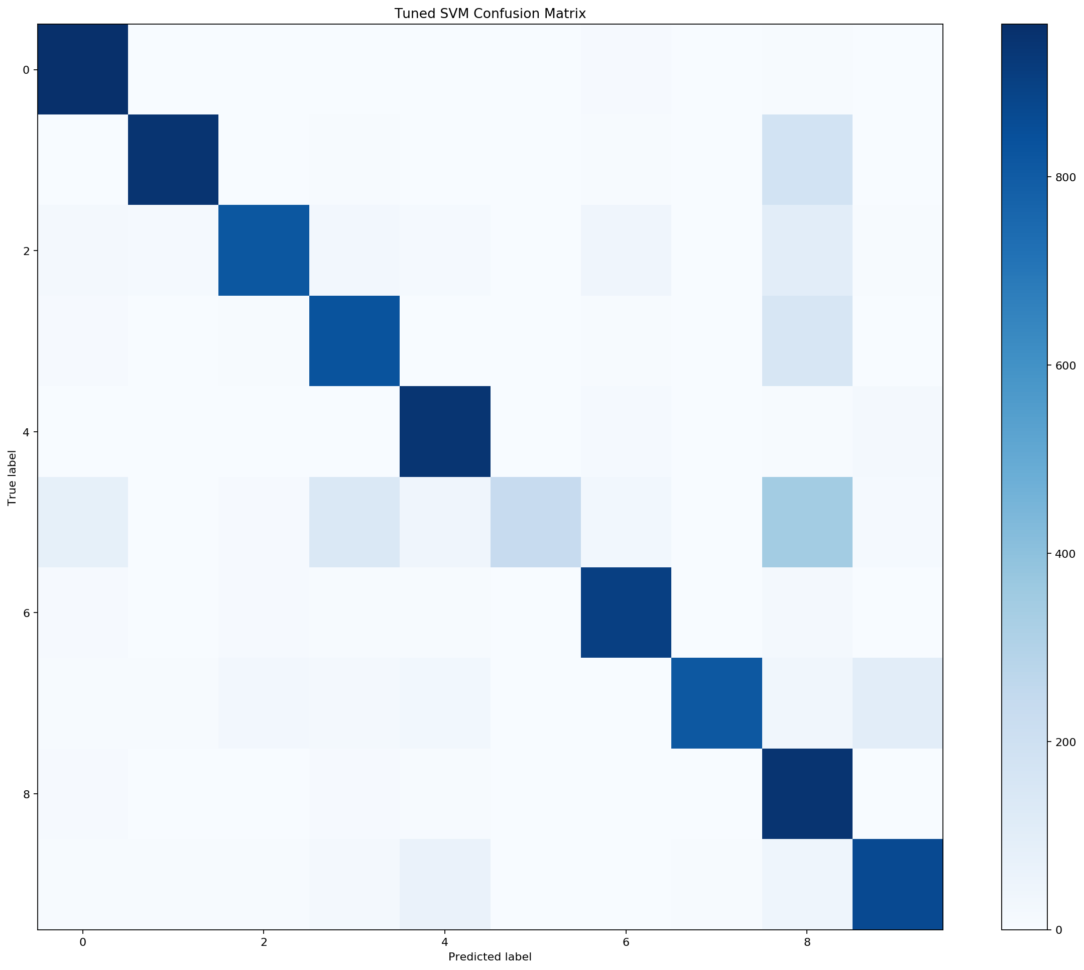
plot_confusion_matrix(cm, title='Tuned SVM Confusion Matrix')
Classification report for classifier SVC(C=5, cache_size=200, class_weight=None, coef0=0.0,
  decision_function_shape='ovr', degree=3, gamma=0.05, kernel='linear',
  max_iter=-1, probability=False, random_state=None, shrinking=True,
  tol=0.001, verbose=False):
              precision    recall  f1-score   support

           0       0.87      0.98      0.92       980
           1       0.97      0.83      0.90      1135
           2       0.93      0.79      0.85      1032
           3       0.79      0.82      0.81      1010
           4       0.86      0.96      0.91       982
           5       1.00      0.26      0.42       892
           6       0.90      0.94      0.92       958
           7       0.98      0.79      0.88      1028
           8       0.52      0.97      0.68       974
           9       0.86      0.86      0.86      1009

   micro avg       0.83      0.83      0.83     10000
   macro avg       0.87      0.82      0.81     10000
weighted avg       0.87      0.83      0.82     10000


Confusion matrix:
[[962   0   1   3   1   0   8   0   5   0]
 [  0 946   3   4   0   0   4   1 177   0]
 [ 19  15 817  25  12   0  38   2 100   4]
 [  8   0   7 832   0   0   4   3 153   3]
 [  1   0   3   1 940   0  13   1   6  17]
 [ 81   2   9 138  38 234  28   2 345  15]
 [ 11   1  11   5   6   1 905   0  18   0]
 [  7   7  25  18  27   0   0 814  31  99]
 [  8   0   1  11   5   0   3   1 944   1]
 [  5   5   5  17  63   0   0   5  43 866]]
Accuracy=0.826
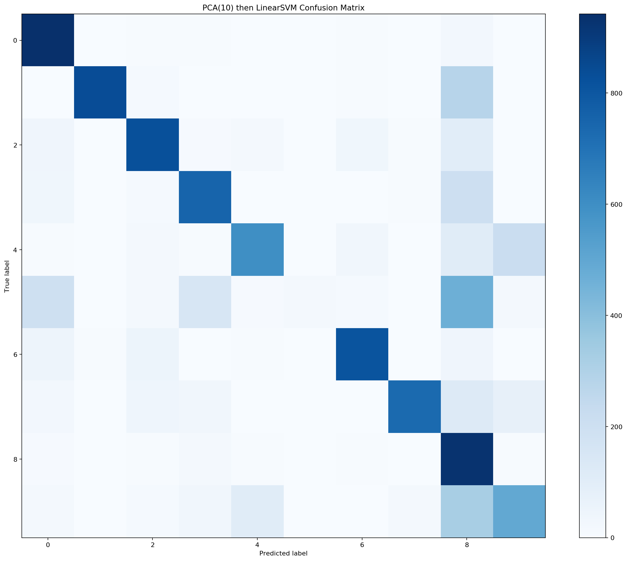
3-信息简化:主成分分析
在运行代价高昂的分类器之前,我们可以从输入数据中提取最少的所需信息吗?
from sklearn.decomposition import PCA
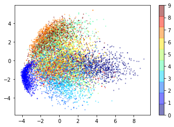
# Let's embedded 28 * 28 = 784 pixels as only 2 dimensions:
pca_2D = '** Add your code here **'
x_train_2D = pca_2D.transform(x_train.reshape(-1, 28 * 28))
x_train_2D.shape
(10000, 2)
pca_2D.explained_variance_ratio_
array([0.09665204, 0.06986566])
plt.scatter(x_train_2D[:, 0], x_train_2D[:, 1], c=y_train[:], edgecolor='none', alpha=0.5,
           cmap=plt.get_cmap('jet', 10), s=5)
plt.colorbar()
<matplotlib.colorbar.Colorbar at 0x10427ca58>
# Embedded images in 10 dimensions:
pca_10D = '** Add your code here **'.fit(x_train.reshape(-1, 28 * 28))
pca_10D
PCA(copy=True, iterated_power='auto', n_components=10, random_state=None,
  svd_solver='auto', tol=0.0, whiten=False)
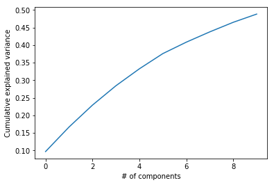
pca_10D.explained_variance_ratio_
array([0.09665204, 0.06986566, 0.06246802, 0.05519677, 0.04828766,
       0.04332001, 0.03256506, 0.0292913 , 0.02727743, 0.02342807])
sum(pca_10D.explained_variance_ratio_)
0.48835202138877953
plt.plot(np.cumsum(pca_10D.explained_variance_ratio_))
plt.xlabel('# of components')
plt.ylabel('Cumulative explained variance')
Text(0, 0.5, 'Cumulative explained variance')
x_train_reduced = pca_10D.transform(x_train.reshape(-1, 28 * 28))
print('What is the dimension of X_train_reduced?')
(10000, 10)
%time clf_faster.fit(x_train_reduced, y_train)
CPU times: user 2.67 s, sys: 15.6 ms, total: 2.69 s
Wall time: 2.69 s
SVC(C=5, cache_size=200, class_weight=None, coef0=0.0,
  decision_function_shape='ovr', degree=3, gamma=0.05, kernel='linear',
  max_iter=-1, probability=False, random_state=None, shrinking=True,
  tol=0.001, verbose=False)
# Validate the model performance: predict the classified digit from the test dataset
%time y_predicted = clf_faster.predict(pca_10D.transform(x_test.reshape(-1, 28 * 28)))
y_predicted
CPU times: user 973 ms, sys: 88.6 ms, total: 1.06 s
Wall time: 675 ms
array([7, 3, 1, ..., 4, 8, 6], dtype=uint8)
print("Classification report for classifier %s:\n%s\n" % (clf_faster, metrics.classification_report(y_test, y_predicted)))
cm = metrics.confusion_matrix(y_test, y_predicted)
print("Confusion matrix:\n%s" % cm)

print("Accuracy={}".format(metrics.accuracy_score(y_test, y_predicted)))
plot_confusion_matrix(cm, title='PCA(10) then LinearSVM Confusion Matrix')
Classification report for classifier SVC(C=5, cache_size=200, class_weight=None, coef0=0.0,
  decision_function_shape='ovr', degree=3, gamma=0.05, kernel='linear',
  max_iter=-1, probability=False, random_state=None, shrinking=True,
  tol=0.001, verbose=False):
              precision    recall  f1-score   support

           0       0.71      0.96      0.82       980
           1       0.99      0.74      0.84      1135
           2       0.83      0.80      0.81      1032
           3       0.75      0.74      0.75      1010
           4       0.80      0.61      0.69       982
           5       0.88      0.02      0.05       892
           6       0.89      0.85      0.87       958
           7       0.96      0.71      0.82      1028
           8       0.36      0.95      0.52       974
           9       0.61      0.49      0.54      1009

   micro avg       0.69      0.69      0.69     10000
   macro avg       0.78      0.69      0.67     10000
weighted avg       0.78      0.69      0.68     10000


Confusion matrix:
[[942   0   5   4   0   0   5   0  23   1]
 [  0 837  12   3   0   0   6   0 277   0]
 [ 39   0 826  11  16   0  34   4 102   0]
 [ 36   2  12 751   0   2   2   4 199   2]
 [  5   1  15   7 597   0  32   2 108 215]
 [195   2  17 151   8  22  13   1 465  18]
 [ 46   5  51   1   6   0 812   0  37   0]
 [ 25   0  43  33   3   1   0 730 119  74]
 [ 10   0   6  15   4   0   4   2 929   4]
 [ 22   0  14  30 108   0   3  16 322 494]]
Accuracy=0.694
4-高级超参数调整:网格搜索
from sklearn.model_selection import GridSearchCV
# We test multiple Gamma and C values:
# gamma_range = np.outer(np.logspace(-3, 0, 4),np.array([1,5])).flatten()
gamma_range = np.outer(np.logspace(-3, 1, 3),np.array([1])).flatten()
gamma_range
array([1.e-03, 1.e-01, 1.e+01])
# We will test on multiple C parameters:
# C_range = np.outer(np.logspace(-3, 3, 7),np.array([1,2, 5]))
# C_range = np.outer(np.logspace(-1, 1, 3), np.array([1, 5])).flatten()
C_range = np.outer(np.logspace(-3, -1, 3), np.array([1])).flatten()
C_range
array([0.001, 0.01 , 0.1 ])
parameters = {'kernel':['linear'], 'C': C_range, 'gamma': gamma_range}
svm_clf = svm.SVC()
grid_clf = '** Add your code here **'
grid_clf
GridSearchCV(cv='warn', error_score='raise-deprecating',
       estimator=SVC(C=1.0, cache_size=200, class_weight=None, coef0=0.0,
  decision_function_shape='ovr', degree=3, gamma='auto_deprecated',
  kernel='rbf', max_iter=-1, probability=False, random_state=None,
  shrinking=True, tol=0.001, verbose=False),
       fit_params=None, iid='warn', n_jobs=4,
       param_grid={'kernel': ['linear'], 'C': array([0.001, 0.01 , 0.1  ]), 'gamma': array([1.e-03, 1.e-01, 1.e+01])},
       pre_dispatch='2*n_jobs', refit=True, return_train_score='warn',
       scoring=None, verbose=2)
%time grid_clf.fit(x_train_small.reshape(-1, 28 * 28), y_train_small)
best_clf = grid_clf.best_estimator_
print('Best hyperparameters founded are:')
grid_clf.best_params_
y_predicted = best_clf.predict(x_test.reshape(-1, 28 * 28))
scores = grid_clf.cv_results_['mean_test_score'].reshape(len(C_range),
                                                     len(gamma_range))
scores
def plot_param_space_heatmap(scores, C_range, gamma_range):
    """https://github.com/ksopyla/svm_mnist_digit_classification/blob/master/mnist_helpers.py#L52"""
    plt.figure(figsize=(8, 6))
    plt.subplots_adjust(left=.2, right=0.95, bottom=0.15, top=0.95)
    plt.imshow(scores, interpolation='nearest', cmap=plt.cm.jet)
    plt.xlabel('gamma')
    plt.ylabel('C')
    plt.colorbar()
    plt.xticks(np.arange(len(gamma_range)), gamma_range, rotation=45)
    plt.yticks(np.arange(len(C_range)), C_range)
    plt.title('Validation accuracy')
    plt.show()
plot_param_space_heatmap(scores, C_range, gamma_range)
# Even easier: TPOT
# https://github.com/EpistasisLab/tpot
from tpot import TPOTClassifier
tpot = TPOTClassifier(generations=5, population_size=50, verbosity=2)
tpot.fit(x_train.reshape(-1, 28 * 28), y_train)
print(tpot.score(x_test.reshape(-1, 28 * 28), y_test))
5-更多机器学习算法
k-近邻
随机森林
LogisticRegression
XGBoost
聚类
更进一步
In-Depth: Support Vector Machines, from the excellent Jake VanderPlas’ Python Data Science Handbook
Hyperparameters and Model Validation, from the excellent Jake VanderPlas’ Python Data Science Handbook
In-Depth: Principal Component Analysis, from the excellent Jake VanderPlas’ Python Data Science Handbook
资源
https://scikit learn.org/stable/auto_examples/classification/plot_digits_classification.htmlsphx-glr自动示例分类图数字分类py
https://github.com/ksopyla/svm_mnist_digit_classification/blob/master/svm_mnist_classification.py