目录
上一个主题


>>> from helper import info; info()
页面更新时间: 2020-02-21 18:15:17
操作系统/OS: Linux-4.19.0-8-amd64-x86_64-with-debian-10.3 ;Python: 3.7.3
11.4. GeoPandas的用法
GeoPandas,基于 Pandas 开发的地理信息分析工具。
页面运行信息
11.4.1. 数据结构
GeoSeries
GeoPandas主要实现两个主要的数据结构,GeoSeries和GeoDataFrame,分别是pandas系列和DataFrame的子类。
GeoSeries本质上是一种向量,向量中的每个条目都对应观察的一组形状。条目可以由一个形状(如单个多边形)组成或由多个形状组成,这些形状被认为是一个观察(例如构成夏威夷州或印度尼西亚等国家的许多多边形)。
geopandas有三个基本类的几何对象(实际上是形状对象):
点/点集合
线/线集合
多边形/多边形集合
请注意,GeoSeries中的所有条目并不是必须为相同的几何类型,但如果类型不同,可能会导致某些操作失败。
①、属性和方法概述
GeoSeries类几乎实现了Shapely对象的所有属性和方法。当应用于GeoSeries时,它们将以元素方式应用于GeoSeries中的所有几何。在两个GeoSeries之间可以应用二进制操作,在这种情况下,操作是按元素进行的。这两个系列将通过匹配索引完成对齐。二进制操作也可以应用于单个几何,在这种情况下,对具有该几何系列的每个元素执行操作。在任一情况下,将酌情返回一个Series或一个GeoSeries。
此处介绍的只是GeoSeries的几个属性和方法的简短摘要,可在所有属性和方法页面中找到完整列表。还有用于扩展现有形状或应用集合理论的一系列操作(例如几何操作中描述的“联合”)来创建新形状。
②、属性
area:形状面积(投影单位)
bounds:每个轴的每个形状的最大与最小坐标元组
total_bounds:整个GeoSeries的每个轴上的最大与最小坐标元组
geom_type:几何类型。
is_valid:测试坐标是否形成合理的几何形状。
③、基本方法
distance(other):返回每个条目到其他条目最小距离的序列
centroid:返回质心的GeoSeries
representative_point():返回位于每个几何中点的GeoSeries。它不返回质心。
to_crs():更改坐标参考系。
plot():绘制GeoSeries。
④、关系测试
geom_almost_equals(other):形状几乎和其他的一样(由于浮点精度问题导致的形状略有不同,效果还是不错的)
contains(other):其他包含的形状
intersects(other):其他相交的形状
11.4.2. 数据结构:GeoDataFrame
GeoDataFrame是一个包含GeoSeries的表格数据结构。
GeoDataFrame最重要的属性是它总是具有一个保存特殊状态的GeoSeries列。此GeoSeries称为GeoDataFrame的“几何”。当空间方法应用于GeoDataFrame(或调用类似区域的空间属性)时,此命令将始终作用于“几何”列。
“geometry”列可通过geometry属性(gdf.geometry)访问,并且可以通过键入gdf.geometry.name的方法找到geometry列名称。
GeoDataFrame还可以包含具有几何(形状)对象的其他列,但每次只能有一个列作为活动式几何。若更改活动式几何列,可使用set_geometry方法。
使用worlds GeoDataFrame的示例:
>>> %matplotlib inline
>>> import geopandas as gpd
>>>
>>> world = gpd.read_file(gpd.datasets.get_path('naturalearth_lowres'))
>>> world.head()
| pop_est | continent | name | iso_a3 | gdp_md_est | geometry | |
|---|---|---|---|---|---|---|
| 0 | 28400000.0 | Asia | Afghanistan | AFG | 22270.0 | POLYGON ((61.21081709172574 35.65007233330923,... |
| 1 | 12799293.0 | Africa | Angola | AGO | 110300.0 | (POLYGON ((16.32652835456705 -5.87747039146621... |
| 2 | 3639453.0 | Europe | Albania | ALB | 21810.0 | POLYGON ((20.59024743010491 41.85540416113361,... |
| 3 | 4798491.0 | Asia | United Arab Emirates | ARE | 184300.0 | POLYGON ((51.57951867046327 24.24549713795111,... |
| 4 | 40913584.0 | South America | Argentina | ARG | 573900.0 | (POLYGON ((-65.50000000000003 -55.199999999999... |
>>> world.plot();

目前,带有国界的名为“geometry”的列是活动几何列:
>>> world.geometry.name
'geometry'
我们也可以将此列重命名为“borders”:
>>> world = world.rename(columns={'geometry': 'borders'}).set_geometry('borders')
>>>
>>> world.geometry.name
'borders'
现在,我们创建质心并使其成为几何列:
>>> world['centroid_column'] = world.centroid
>>>
>>> world = world.set_geometry('centroid_column')
>>>
>>> world.plot();
注意:GeoDataFrame可根据名称跟踪活动列,因此若重命名活动几何列,则还必须重置几何项:
gdf = gdf.rename(columns={'old_name': 'new_name'}).set_geometry('new_name')
默认情况下,当您使用read_file命令时,文件中的空间对象列在默认情况下被命名为“geometry”,并将其设置为活动几何列。但是,尽管对列的名称和跟踪活动列的特殊属性名称使用的是相同术语,但其实它们是不同的。您可以使用set_geometry命令将活动几何列转移到不同的GeoSeries。此外,gdf.geometry将始终返回活动几何列,而不是返回geometry列。如果想调用“geometry”的列,并且是不同的活动几何列,请使用gdf [‘geometry’],而不是gdf.geometry。 ### ①、属性和方法
GeoSeries所描述的任何属性调用或方法都可以在GeoDataFrame上工作,实际上,它们只是应用于“几何”GeoSeries。
11.4.3. 读取空间数据
geopandas可以读取任意基于矢量的空间数据格式,包括ESRI shapefile,GeoJSON文件等命令:
gpd.read_file()
它返回一个GeoDataFrame对象。 (这是可能的,因为geopandas利用的是fiona库,并且利用的是大规模的开源程序GDAL / OGR,以促进空间数据转换)。
在read_file()文件后输出的任何参数将被输出列fiona.open中,其实是数据导入的工作。
>>> import fiona
一般来说,read_file很有用的,通常会生成你想要的参数,但如果遇到瓶颈,请输入:
help(fiona.open)
其中,可以使用driver关键字显式设置驱动程序(shapefile,GeoJSON),或者使用layer关键字从多层文件中筛选中单个图层。
geopandas也可以使用read_postgis()命令从PostGIS数据库中获取数据。
11.4.4. 写入空间数据
GeoDataFrames可以使用GeoDataFrame.to_file()方法导出许多不同的标准格式。若查看支持的完整格式列表,请键入import fiona; fiona.supported_drivers。
11.4.5. 地图工具
geopandas提供了一个用于制作地图的高级接口matplotlib库。其映射形状与GeoSeries或GeoDataFrame使用plot()方法一样便于操作。
一些示例数据:
>>> %matplotlib inline
>>> import geopandas as gpd
>>> world = gpd.read_file(gpd.datasets.get_path('naturalearth_lowres'))
>>>
>>> cities = gpd.read_file(gpd.datasets.get_path('naturalearth_cities'))
我们现在可以绘制这些GeoDataFrames:
>>> # Examine country GeoDataFrame
>>> world.head()
| pop_est | continent | name | iso_a3 | gdp_md_est | geometry | |
|---|---|---|---|---|---|---|
| 0 | 28400000.0 | Asia | Afghanistan | AFG | 22270.0 | POLYGON ((61.21081709172574 35.65007233330923,... |
| 1 | 12799293.0 | Africa | Angola | AGO | 110300.0 | (POLYGON ((16.32652835456705 -5.87747039146621... |
| 2 | 3639453.0 | Europe | Albania | ALB | 21810.0 | POLYGON ((20.59024743010491 41.85540416113361,... |
| 3 | 4798491.0 | Asia | United Arab Emirates | ARE | 184300.0 | POLYGON ((51.57951867046327 24.24549713795111,... |
| 4 | 40913584.0 | South America | Argentina | ARG | 573900.0 | (POLYGON ((-65.50000000000003 -55.199999999999... |
>>> world.plot();

注意,一般来说,任何可以输出到matplotlib中pyplot的选项(或者适用于行的样式选项)都可以输出给plot()方法。
Chloropleth地图
geopandas创建Chloropleth地图比较简单(每个形状颜色对应于相关联变量值的地图)。只需使用plot命令,将列参数设置为要用于分配颜色值的列即可。
>>> # Plot by GDP per capta
>>> world = world[(world.pop_est>0) & (world.name!="Antarctica")]
>>>
>>> world['gdp_per_cap'] = world.gdp_md_est / world.pop_est
>>>
>>> world.plot(column='gdp_per_cap');
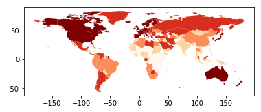
选择颜色。 还可以使用cmap选项修改plot颜色(有关色彩图的完整列表,请参阅matplotlib网站):
>>> world.plot(column='gdp_per_cap', cmap='OrRd');
颜色映射的缩放方式也可以使用scheme选项(如果你已经安装了pysal,可以通过conda install pysal来实现)。默认情况下,scheme设置为“equal_intervals”,但也可以调整为任何其他pysal选项,如“分位数”,“百分位数”等。
>>> world.plot(column='gdp_per_cap', cmap='OrRd', scheme='quantiles');
/usr/lib/python3/dist-packages/pysal/__init__.py:65: VisibleDeprecationWarning: PySAL's API will be changed on 2018-12-31. The last release made with this API is version 1.14.4. A preview of the next API version is provided in the pysalnext package. The API changes and a guide on how to change imports is provided at https://migrating.pysal.org
  ), VisibleDeprecationWarning)
/usr/lib/python3/dist-packages/scipy/stats/stats.py:1713: FutureWarning: Using a non-tuple sequence for multidimensional indexing is deprecated; use arr[tuple(seq)] instead of arr[seq]. In the future this will be interpreted as an array index, arr[np.array(seq)], which will result either in an error or a different result.
  return np.add.reduce(sorted[indexer] * weights, axis=axis) / sumval
地图图层
在合并地图之前,请一定要确保它们的共享公用CRS(以便它们对齐)。
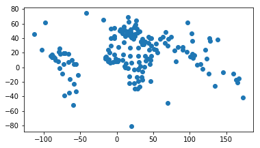
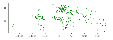
>>> # Look at capitals
>>> # Note use of standard `pyplot` line style options
>>> cities.plot(marker='*', color='green', markersize=5);
>>>
>>> # Check crs
>>> cities = cities.to_crs(world.crs)
>>>
>>> # Now we can overlay over country outlines
>>> # And yes, there are lots of island capitals
>>> # apparently in the middle of the ocean!
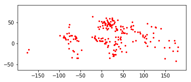
方法1
>>> base = world.plot(color='white')
>>>
>>> cities.plot(ax=base, marker='o', color='red', markersize=5);
使用matplotlib对象
>>> import matplotlib.pyplot as plt
>>>
>>> fig, ax = plt.subplots()
>>>
>>> # set aspect to equal. This is done automatically
>>> # when using *geopandas* plot on it's own, but not when
>>> # working with pyplot directly.
>>>
>>> ax.set_aspect('equal')
>>>
>>> world.plot(ax=ax, color='white')
<matplotlib.axes._subplots.AxesSubplot at 0x7fd31a52bc50>
>>> cities.plot(ax=ax, marker='o', color='red', markersize=5)
<matplotlib.axes._subplots.AxesSubplot at 0x7fd31a52bc50>
<Figure size 432x288 with 0 Axes>
>>>
>>>
>>> fig, ax = plt.subplots()
>>>
>>> # set aspect to equal. This is done automatically
>>> # when using *geopandas* plot on it's own, but not when
>>> # working with pyplot directly.
>>>
>>> ax.set_aspect('equal')
>>>
>>> world.plot(ax=ax, color='white')
>>>
>>>
>>> cities.plot(ax=ax, marker='o', color='red', markersize=5)
>>>
>>> plt.show();

管理投影
1.坐标参考系统
CRS非常重要,其意义在于GeoSeries或GeoDataFrame对象中的几何形状是任意空间中的坐标集合。 CRS可以使Python的坐标与地球上的具体实物点相关联。
使用proj4字符串代码的方法引用CRS。你可以从www.spatialreference.org或remotesensing.org找到最常用的代码。
例如,最常用的CRS之一是WGS84纬度 - 经度投影。这个投影的proj4表示通常可以用多种不同的方式引用相同CRS:
"+proj=longlat +ellps=WGS84 +datum=WGS84 +no_defs"
通用的投影可以通过EPSG代码来引用,因此这个通用的投影也可以使用proj4字符串调用
"+init=epsg:4326".
geopandas包含有CRS的表示方法,包括proj4字符串本身
("+proj=longlat +ellps=WGS84 +datum=WGS84 +no_defs")
或在字典中分解的参数:
{'proj': 'latlong', 'ellps': 'WGS84', 'datum': 'WGS84', 'no_defs': True}
此外,也可直接采用EPSG代码完成一些功能。
以下为参考值,是一些非常常见的投影和它们的proj4字符串:
WGS84纬度/经度:“+ proj = longlat + ellps = WGS84 + datum = WGS84 + no_defs”或“+ init = epsg:4326”
UTM区域(北):“+ proj = utm + zone = 33 + ellps = WGS84 + datum = WGS84 + units = m + no_defs”
UTM Zones(南):“+ proj = utm + zone = 33 + ellps = WGS84 + datum = WGS84 + units = m + no_defs + south”
2.设置投影
投影有两个操作方法:设置投影和重新投影。
当地理坐标有坐标数据(x-y值),但没有关于这些坐标如何指向实际位置的信息时,需要设置投影。如果没有设置CRS,地理信息的几何操作虽可以工作,但不会变换坐标,导出的文件也可能无法被其他软件正常理解。
注意,大多数情况你不需要设置投影。使用from_file()命令加载的数据会始终包括投影信息。您可以通过crs属性来查看当前CRS对象:my_geoseries.crs。
然而,您可能会获得不包含投影的数据。在这种情况下,您必须设置CRS,以便地理数据库作出解释坐标的合理操作。
例如,将纬度和经度的电子表格手动转换为GeoSeries,可以通过WGS84纬度 - 经度CRS分配给crs属性的方法来设置投影:
my_geoseries.crs = {'init' :'epsg:4326'}
3.重新投影
重新投影是从一个坐标系变到另一个坐标系并重新表示位置的过程。地球上的任意一点放置到二维平面上时,所有投影都是失真的,您应用最好的投影可能不同于与您导入的数据相关联的投影。在这些情况下,可以使用to_crs命令重新进行投影:
>>> # load example data
>>> world = gpd.read_file(gpd.datasets.get_path('naturalearth_lowres'))
>>>
>>> # Check original projection
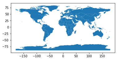
>>> # (it's Platte Carre! x-y are long and lat)
>>> world.crs
{'init': 'epsg:4326'}
>>> # Visualize
>>> world.plot()
<matplotlib.axes._subplots.AxesSubplot at 0x7fd31772e828>
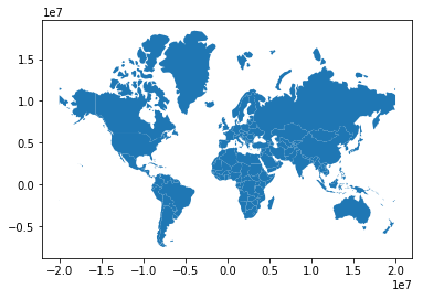
>>> # Reproject to Mercator (after dropping Antartica)
>>> world = world[(world.name != "Antarctica") & (world.name != "Fr. S. Antarctic Lands")]
>>> world = world.to_crs({'init': 'epsg:3395'}) # world.to_crs(epsg=3395) would also work
>>> world.plot();
11.4.6. 五、几何操作
geopandas在shapely库中提供了所有几何操作的工具。
请注意,所有用于创建不同空间数据集(如创建交叉点或差异)新形状的集合理论工具的文档可以在设置操作页面上查找。
1、创建方法
GeoSeries.buffer(distance, resolution=16)
返回每个几何对象的给定距离内的所有点的GeoSeries。
GeoSeries.boundary
返回每个几何的集合理论边界的低维对象GeoSeries。
GeoSeries.centroid
返回每个几何质心的点GeoSeries。
GeoSeries.convex_hull
返回包含每个对象所有点的最小凸多边形的几何体的GeoSeries,除非对象中的点数小于三。对于两个点,凸多边形返货的是一个LineString;若为1,则表示一个点。
GeoSeries.envelope
返回包含每个对象点的最小矩形(平行于坐标轴的边)的几何体的GeoSeries。
GeoSeries.simplify(tolerance, preserve_topology=True)
返回包含每个对象简化表示的GeoSeries。
GeoSeries.unary_union
返回包含GeoSeries中所有几何并集的GeoSeries。
2、仿射变换
GeoSeries.rotate(self, angle, origin='center', use_radians=False)
旋转GeoSeries坐标。
GeoSeries.scale(self, xfact=1.0, yfact=1.0, zfact=1.0, origin='center')
沿每个(x,y,z)维度缩放GeoSeries几何。
GeoSeries.skew(self, angle, origin='center', use_radians=False)
通过沿x和y维度的角度剪切或倾斜GeoSeries的几何图形。
GeoSeries.translate(self, angle, origin='center', use_radians=False)
移动GeoSeries的坐标。
3、几何操作的示例
>>> %matplotlib inline
>>>
>>> import geopandas as gpd
>>> from geopandas import GeoDataFrame
>>> from shapely.geometry import Polygon
>>> from geopandas import GeoSeries
>>> p1 = Polygon([(0, 0), (1, 0), (1, 1)])
>>> p2 = Polygon([(0, 0), (1, 0), (1, 1), (0, 1)])
>>> p3 = Polygon([(2, 0), (3, 0), (3, 1), (2, 1)])
>>> g = GeoSeries([p1, p2, p3])
>>>
返回正常的pandas对象。GeoSeries的area属性将返回包含GeoSeries中每个项目的区域的pandas.Series:
>>> print (g.area)
0    0.5
1    1.0
2    1.0
dtype: float64
返回GeoPandas对象:
>>> g.buffer(0.5)
0    POLYGON ((-0.3535533905932737 0.35355339059327...
1    POLYGON ((-0.5 0, -0.5 1, -0.4975923633360985 ...
2    POLYGON ((1.5 0, 1.5 1, 1.502407636663901 1.04...
dtype: object
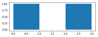
GeoPandas使用的是descartes方法生成matplotlib图。要生成我们自己的GeoSeries图,请使用:
>>> g.plot()
<matplotlib.axes._subplots.AxesSubplot at 0x7fd3175e23c8>
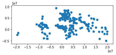
为了演示更复杂的操作,我们将生成一个包含2000个随机点的GeoSeries:
>>> from shapely.geometry import Point
>>> import numpy as np
>>> xmin, xmax, ymin, ymax = 900000, 1080000, 120000, 280000
>>> xc = (xmax - xmin) * np.random.random(2000) + xmin
>>> yc = (ymax - ymin) * np.random.random(2000) + ymin
>>> pts = GeoSeries([Point(x, y) for x, y in zip(xc, yc)])
现在在每个点周围画一个固定半径的圆:
>>> circles = pts.buffer(2000)
我们可以将这些圆形折叠成一个单一的多边形
>>> mp = circles.unary_union
11.4.7. 六、使用覆盖设置操作
当使用多个空间数据集(尤其是多个多边形或线数据集)时,用户通常想用这些重叠(或不重叠)位置的数据集创建新的形状。这些操作通常使用的是交集集合,通过联合和差异的方法来引用。可通过overlay 函数在geopandas库中操作。
覆盖的DataFrame级别并不是在单个几何体上操作,而是两者的属性都保留。实际上,对于第一个GeoDataFrame中形状来说,此操作针对于其他GeoDataFrame中的每个形状执行:
(熟悉shapely库的用户的请注意:overlay可以被认为是提供标准形状操作的版本,对于处理两个GeoSeries应用集合操作的复杂性来讲,标准的形状集合操作也可以作为GeoSeries方法。)
1、不同的Overlay操作
首先,我们创建一些示例数据:
>>>
>>> from shapely.geometry import Polygon
>>>
>>> polys1 = gpd.GeoSeries([Polygon([(0,0), (2,0), (2,2), (0,2)]),
>>>                        Polygon([(2,2), (4,2), (4,4), (2,4)])])
>>>
>>>
>>> polys2 = gpd.GeoSeries([Polygon([(1,1), (3,1), (3,3), (1,3)]),
>>>                          Polygon([(3,3), (5,3), (5,5), (3,5)])])
>>>
>>>
>>> df1 = gpd.GeoDataFrame({'geometry': polys1, 'df1':[1,2]})
>>> df2 = gpd.GeoDataFrame({'geometry': polys2, 'df2':[1,2]})
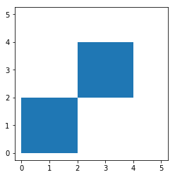
这两个GeoDataFrames有一些重叠区域:
>>> ax = df1.plot(color='red');
>>>
>>> df2.plot(ax=ax, color='green');
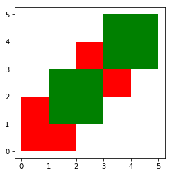
上面的例子说明是的覆盖模式。覆盖函数是通过覆盖GeoDataFrames的方法来确定所有单个几何的集合。此结果覆盖由两个输入GeoDataFrames覆盖的区域组成,保留着两个GeoDataFrames组合边界定义的唯一区域。
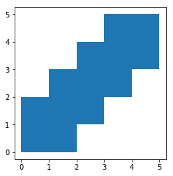
当使用how =’union’时,将返回所有可能的几何体:
>>> res_union = gpd.overlay(df1, df2, how='union')
>>>
>>> res_union
| df1 | df2 | geometry | |
|---|---|---|---|
| 0 | 1.0 | 1.0 | POLYGON ((1 2, 2 2, 2 1, 1 1, 1 2)) |
| 1 | 2.0 | 1.0 | POLYGON ((2 2, 2 3, 3 3, 3 2, 2 2)) |
| 2 | 2.0 | 2.0 | POLYGON ((3 4, 4 4, 4 3, 3 3, 3 4)) |
| 3 | 1.0 | NaN | POLYGON ((0 0, 0 2, 1 2, 1 1, 2 1, 2 0, 0 0)) |
| 4 | 2.0 | NaN | (POLYGON ((2 3, 2 4, 3 4, 3 3, 2 3)), POLYGON ... |
| 5 | NaN | 1.0 | (POLYGON ((1 2, 1 3, 2 3, 2 2, 1 2)), POLYGON ... |
| 6 | NaN | 2.0 | POLYGON ((3 4, 3 5, 5 5, 5 3, 4 3, 4 4, 3 4)) |
>>> ax = res_union.plot()
>>>
>>> df1.plot(ax=ax, facecolor='none');
>>>
>>> df2.plot(ax=ax, facecolor='none');
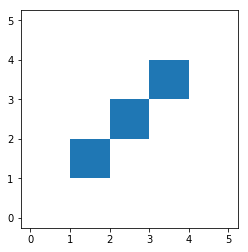
其他操作将返回那些几何的不同子集。使用how =’intersection’方法,返回的是两个GeoDataFrames包含的几何体:
>>> res_intersection = gpd.overlay(df1, df2, how='intersection')
>>>
>>> res_intersection
| df1 | df2 | geometry | |
|---|---|---|---|
| 0 | 1 | 1 | POLYGON ((1 2, 2 2, 2 1, 1 1, 1 2)) |
| 1 | 2 | 1 | POLYGON ((2 2, 2 3, 3 3, 3 2, 2 2)) |
| 2 | 2 | 2 | POLYGON ((3 4, 4 4, 4 3, 3 3, 3 4)) |
>>> ax = res_intersection.plot()
>>>
>>> df1.plot(ax=ax, facecolor='none');
>>>
>>> df2.plot(ax=ax, facecolor='none');
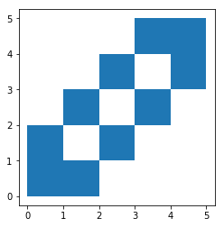
how =’symmetric_difference’与’intersection’相反,返回的几何只是GeoDataFrames其中之一的一部分,并不是两者的一部分:
>>> res_symdiff = gpd.overlay(df1, df2, how='symmetric_difference')
>>>
>>> res_symdiff
| df1 | df2 | geometry | |
|---|---|---|---|
| 0 | 1.0 | NaN | POLYGON ((0 0, 0 2, 1 2, 1 1, 2 1, 2 0, 0 0)) |
| 1 | 2.0 | NaN | (POLYGON ((2 3, 2 4, 3 4, 3 3, 2 3)), POLYGON ... |
| 2 | NaN | 1.0 | (POLYGON ((1 2, 1 3, 2 3, 2 2, 1 2)), POLYGON ... |
| 3 | NaN | 2.0 | POLYGON ((3 4, 3 5, 5 5, 5 3, 4 3, 4 4, 3 4)) |
>>> ax = res_symdiff.plot()
>>>
>>> df1.plot(ax=ax, facecolor='none');
>>>
>>> df2.plot(ax=ax, facecolor='none');
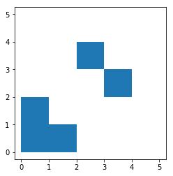
作为df1的一部分但此部分并不包含在df2中,要获取这样的几何体,可以使用how =’difference’方法:
>>> res_difference = gpd.overlay(df1, df2, how='difference')
>>>
>>> res_difference
| geometry | df1 | |
|---|---|---|
| 0 | POLYGON ((0 0, 0 2, 1 2, 1 1, 2 1, 2 0, 0 0)) | 1 |
| 1 | (POLYGON ((2 3, 2 4, 3 4, 3 3, 2 3)), POLYGON ... | 2 |
>>> ax = res_difference.plot()
>>>
>>> df1.plot(ax=ax, facecolor='none');
>>>
>>> df2.plot(ax=ax, facecolor='none');
最后,使用how =’identity’方法生成的,结果由df1的表面组成。若想获得df2覆盖df1的几何体,可使用以下方法:
>>> res_identity = gpd.overlay(df1, df2, how='identity')
>>>
>>> res_identity
>>>
| df1 | df2 | geometry | |
|---|---|---|---|
| 0 | 1.0 | 1.0 | POLYGON ((1 2, 2 2, 2 1, 1 1, 1 2)) |
| 1 | 2.0 | 1.0 | POLYGON ((2 2, 2 3, 3 3, 3 2, 2 2)) |
| 2 | 2.0 | 2.0 | POLYGON ((3 4, 4 4, 4 3, 3 3, 3 4)) |
| 3 | 1.0 | NaN | POLYGON ((0 0, 0 2, 1 2, 1 1, 2 1, 2 0, 0 0)) |
| 4 | 2.0 | NaN | (POLYGON ((2 3, 2 4, 3 4, 3 3, 2 3)), POLYGON ... |
>>> ax = res_identity.plot()
>>>
>>> df1.plot(ax=ax, facecolor='none');
>>>
>>> df2.plot(ax=ax, facecolor='none');
2、覆盖国家的示例
首先,我们加载国家和城市示例数据集,然后选择:
>>> world = gpd.read_file(gpd.datasets.get_path('naturalearth_lowres'))
>>>
>>> capitals = gpd.read_file(gpd.datasets.get_path('naturalearth_cities'))
>>>
>>> # Select South Amarica and some columns
>>> countries = world[world['continent'] == "South America"]
>>>
>>> countries = countries[['geometry', 'name']]
>>>
>>> # Project to crs that uses meters as distance measure
>>> countries = countries.to_crs('+init=epsg:3395')
>>>
>>> capitals = capitals.to_crs('+init=epsg:3395')
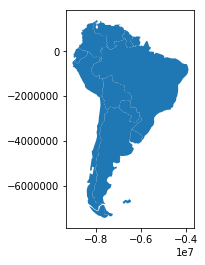
为了说明overlay 功能,我们来假设以下情况,使用国家的GeoDataFrame和大写的GeoDataFrame来识别每个国家的“核心”部分(定义在首都500km内的区域)。
>>> # Look at countries:
>>> countries.plot();
>>>
>>> # Now buffer cities to find area within 500km.
>>> # Check CRS -- World Mercator, units of meters.
>>> capitals.crs
>>>
>>>
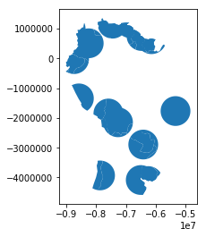
>>> # make 500km buffer
>>> capitals['geometry']= capitals.buffer(500000)
>>>
>>> capitals.plot();
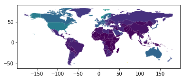
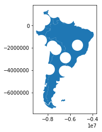
仅选择距离首都500公里内的国家部分,我们指定的如何选项是“intersect”,这将创建一组新的多边形,其中这两个层是重叠的:
>>> country_cores = gpd.overlay(countries, capitals, how='intersection')
>>> country_cores.plot();
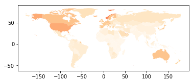
更改“方式”选项可允许不同类型的重叠操作。例如,我们对远离国家首都的部分感兴趣,可以计算两者的差异。
>>> country_peripheries = gpd.overlay(countries, capitals, how='difference')
>>> country_peripheries.plot();
11.4.8. 七、溶解聚集
通常情况下,我们发现自己使用的空间数据比我们需要的粒度更细。例如,我们有国家地方单位的数据,但我们感兴趣的是研究国家层面的模式。
在非空间设置中,我们使用groupby函数聚合数据。但是使用空间数据时,可能会需要一个特殊的工具,也可以聚合几何特征。在geopandas库中,该功能由dissolve函数提供。
dissolve可以做三件事情:(a)它将给定组中的所有几何图形,并一起溶解成单个几何特征(使用unary_union方法);(b)它聚合组中的所有数据行,使用的是groupby.aggregate()方法;(c)将以上这两种方法结合。
1、dissolve示例
假设我们对研究大陆感兴趣,但我们只有国家级数据。我们可以轻松地将其转换为大陆级数据集。
首先,我们只需要大陆形状和名称。默认情况下,dissolve将’first’输出到groupby.aggregate。
>>> world = gpd.read_file(gpd.datasets.get_path('naturalearth_lowres'))
>>>
>>> world = world[['continent', 'geometry']]
>>>
>>> continents = world.dissolve(by='continent')
>>>
>>> continents.plot();
>>>
>>> continents.head()
| geometry | |
|---|---|
| continent | |
| Africa | (POLYGON ((49.54351891459575 -12.4698328589405... |
| Antarctica | (POLYGON ((-159.2081835601977 -79.497059421708... |
| Asia | (POLYGON ((120.7156087586305 -10.2395813940878... |
| Europe | (POLYGON ((-52.55642473001839 2.50470530843705... |
| North America | (POLYGON ((-61.68000000000001 10.76, -61.105 1... |

11.4.9. 合并数据
有两种方法可以合并地理数据库中数据集中的属性连接和空间连接。
在属性连接中,GeoSeries或GeoDataFrame与基于常见变量的常规pandas Series或DataFrame组合。有类似于普通合并或加入pandas。
在空间连接中,由于GeoSeries与GeoDataFrames彼此的空间关系而被组合。
在下面的示例中,我们使用这些数据集:
>>> %matplotlib inline
>>> import geopandas as gpd
>>>
>>> world = gpd.read_file(gpd.datasets.get_path('naturalearth_lowres'))
>>>
>>> cities = gpd.read_file(gpd.datasets.get_path('naturalearth_cities'))
>>>
>>> # For attribute join
>>> country_shapes = world[['geometry', 'iso_a3']]
>>>
>>> country_names = world[['name', 'iso_a3']]
>>>
>>> # For spatial join
>>> countries = world[['geometry', 'name']]
>>>
>>> countries = countries.rename(columns={'name':'country'})
属性连接
属性连接可使用merge方法完成。通常,建议使用空间数据集调用merge的方法。如果GeoDataFrame在left参数中,merge函数将独立工作;如果DataFrame在left参数中,并且GeoDataFrame在right的位置,那么结果将不再是GeoDataFrame。
通过与pandas DataFrame合并,为GeoDataFrame添加全名的方法,该GeoDataFrame会具有每个国家/地区的ISO代码。
>>> # country_shapes` is GeoDataFrame with country shapes and iso codes
>>>
>>> country_shapes.head()
| geometry | iso_a3 | |
|---|---|---|
| 0 | POLYGON ((61.21081709172574 35.65007233330923,... | AFG |
| 1 | (POLYGON ((16.32652835456705 -5.87747039146621... | AGO |
| 2 | POLYGON ((20.59024743010491 41.85540416113361,... | ALB |
| 3 | POLYGON ((51.57951867046327 24.24549713795111,... | ARE |
| 4 | (POLYGON ((-65.50000000000003 -55.199999999999... | ARG |
>>> country_names.head()
| name | iso_a3 | |
|---|---|---|
| 0 | Afghanistan | AFG |
| 1 | Angola | AGO |
| 2 | Albania | ALB |
| 3 | United Arab Emirates | ARE |
| 4 | Argentina | ARG |
>>> country_shapes = country_shapes.merge(country_names, on='iso_a3')
>>>
>>> country_shapes.head()
| geometry | iso_a3 | name | |
|---|---|---|---|
| 0 | POLYGON ((61.21081709172574 35.65007233330923,... | AFG | Afghanistan |
| 1 | (POLYGON ((16.32652835456705 -5.87747039146621... | AGO | Angola |
| 2 | POLYGON ((20.59024743010491 41.85540416113361,... | ALB | Albania |
| 3 | POLYGON ((51.57951867046327 24.24549713795111,... | ARE | United Arab Emirates |
| 4 | (POLYGON ((-65.50000000000003 -55.199999999999... | ARG | Argentina |
空间连接
在空间联接中,两个几何对象基于它们彼此的空间关系而被合并。
>>> # One GeoDataFrame of countries, one of Cities.
>>> # Want to merge so we can get each city's country.
>>> countries.head()
| geometry | country | |
|---|---|---|
| 0 | POLYGON ((61.21081709172574 35.65007233330923,... | Afghanistan |
| 1 | (POLYGON ((16.32652835456705 -5.87747039146621... | Angola |
| 2 | POLYGON ((20.59024743010491 41.85540416113361,... | Albania |
| 3 | POLYGON ((51.57951867046327 24.24549713795111,... | United Arab Emirates |
| 4 | (POLYGON ((-65.50000000000003 -55.199999999999... | Argentina |
>>> cities.head()
| name | geometry | |
|---|---|---|
| 0 | Vatican City | POINT (12.45338654497177 41.90328217996012) |
| 1 | San Marino | POINT (12.44177015780014 43.936095834768) |
| 2 | Vaduz | POINT (9.516669472907267 47.13372377429357) |
| 3 | Luxembourg | POINT (6.130002806227083 49.61166037912108) |
| 4 | Palikir | POINT (158.1499743237623 6.916643696007725) |
>>> cities_with_country = gpd.sjoin(cities, countries, how="inner", op='intersects')
>>>
>>> cities_with_country.head()
| name | geometry | index_right | country | |
|---|---|---|---|---|
| 0 | Vatican City | POINT (12.45338654497177 41.90328217996012) | 79 | Italy |
| 1 | San Marino | POINT (12.44177015780014 43.936095834768) | 79 | Italy |
| 192 | Rome | POINT (12.481312562874 41.89790148509894) | 79 | Italy |
| 2 | Vaduz | POINT (9.516669472907267 47.13372377429357) | 9 | Austria |
| 184 | Vienna | POINT (16.36469309674374 48.20196113681686) | 9 | Austria |