Actinia Quickstart¶

Actinia是一个开源的restapi，用于地理数据的可伸缩、分布式、高性能处理，它使用grassgis完成计算任务。Actinia提供了一个restapi来处理卫星图像、卫星图像的时间序列、栅格和矢量数据。

Contents

ace简介-actinia命令执行
设置您的环境
访问示例数据
- 从外部源访问数据
提交前检查剩余呼叫
显示地图-地图渲染
脚本示例
尝试的东西
- 创建新位置
- 安装GRASS GIS插件（扩展）
接下来呢？

锕系元素有不同的用途：

curl 或类似的命令行工具
这个 Postman 浏览器扩展
打开GRASS GIS会话并使用 ace （actinia命令执行）工具
REST API的其他接口

在这个快速入门中，我们利用GRASS-GIS方便地从会话启动命令到actinia服务器（actinia服务器本身使用GRASS-GIS）。其思想是在本地快速开发一个小数据集上的工作流，然后在服务器上执行它。

ace简介-actinia命令执行 ¶

这个 ace 工具 (details )允许在actinia REST服务上执行单个GRASS GIS命令或GRASS GIS命令列表(https://actinia.mundialis.de/). 此外，它还提供作业管理、列出用户可以访问的位置、地图集和地图图层的功能，以及地图集的创建和删除。

第 ace 工具必须在活动的GRASS GIS会话中执行，并将使用此会话的当前位置访问actinia服务。

当前位置设置可以被重写 --location LOCATION_NAME 选项。默认情况下，所有命令都将在 短暂的 数据库。因此，必须使用增强的GRASS命令导出生成的输出。

选择权 --persistent MAPSET_NAME 允许在中执行命令 持久的 用户数据库。它可以与 --location LOCATION_NAME 选项。

设置您的环境 ¶

用户必须设置以下环境变量以指定actinia服务器和凭据：

# set credentials and REST server URL
export ACTINIA_USER='demouser'
export ACTINIA_PASSWORD='gu3st!pa55w0rd'
export ACTINIA_URL='https://actinia.mundialis.de/latest'

访问示例数据 ¶

选定的数据集可供演示用户使用。要列出您可以访问的位置，请运行

ace --list-locations
['latlong', 'nc_spm_08', 'utm_32n', 'latlong']

以下命令列出了当前GRASS GIS会话（nc_spm_08）中当前位置的地图集：

# running ace in the "nc_spm_08" location:
ace --list-mapsets
['PERMANENT', 'landsat']

从外部源访问数据 ¶

GRASS-GIS命令可以通过actinia-specific扩展进行扩充。这个 + 可以为输入参数指定运算符，以导入位于web上的资源并指定输出参数的导出。

重要的是，本地位置和映射集的名称必须与actinia REST服务器上的名称相对应。

目前可用的数据集有（按预测组织）：

北卡罗来纳州样本数据集（NC州平面公制CRS，EPSG:3358）：
- 基础制图 (nc_spm_08/PERMANENT ；来源：https://grassbook.org/datasets/datasets-3rd-edition/)
- 陆地卫星次中心 (nc_spm_08/landsat ；来源：https://grass.osgeo.org/download/data/)
经纬度位置（LatLong WGS84，爱普生：4326):
- 空的 (latlong/PERMANENT/ ）
- 16天NDVI，MOD13C1，V006，CMG 0.05度分辨率。 (latlong/modis_ndvi_global/ ；来源：https://lpdaac.usgs.gov/products/mod13c1v006/)
- 2017亚洲第一届成长学位日 (latlong/asia_gdd_2017/ ；来源：https://www.mundailis.de/en/temperature-data/)
- 2017亚洲第一届热带日 (latlong/asia_tropical_2017/ ）
- 2017年亚洲每日温度，包括最低温度、最高温度和平均温度 (latlong/asia_lst_daily_2017/ ）
欧洲（EU LAEA CRS，爱普生：3035):
- 欧盟2500万德国马克V1.1 (eu_laea/PERMANENT/ ；来源：https://land.copernicus.eu/images-in-site/eu-dem)
- 2012年科林土地覆盖率，g100 (eu_laea/corine_2012/ ；来源：https://land.copernicus.eu/pan-european/corine-land-cover/clc-2012)
世界穆尔韦德（EPSG 54009）：
- GHS_POP_GPW42015_GLOBE_R2015A_54009_250_v1_0 (world_mollweide/pop_jrc ；来源：https://ghsl.jrc.ec.europa.eu/ghs_pop.php)

提交前检查剩余呼叫 ¶

要生成actinia process chain JSON请求，只需添加–dry run标志：

ace --dry-run r.slope.aspect elevation=elevation slope=myslope

显示地图-地图渲染 ¶

渲染地图非常容易（而且很快）：

# check amount of pixels, just FYI
ace --location latlong r.info globcover@globcover
ace --location latlong --render-raster globcover@globcover

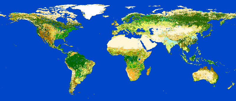
由actinia提供的ESA全球覆盖图

短暂加工是猕猴桃的默认加工方法。命令在一个短暂的映射集中执行，处理后将删除该映射集。您可以导出GRASS GIS模块的输出，以存储计算结果以供下载和进一步分析。当前支持以下导出格式：

栅格： GTiff
矢量： ESRI_Shapefile ， GeoJSON ， GML
table: CSV, TXT

脚本示例 ¶

示例1：从高程模型计算坡度和坡向以及单变量统计信息 ¶

以下命令（存储在脚本中并使用 ace )将从internet源导入栅格图层作为栅格地图 elev ，将计算区域设置为地图并计算坡度。有关栅格图层的其他信息可通过 r.info .

将以下脚本存储为文本文件 ace_dtm_statistics.sh ：

# grass77 ~/grassdata/nc_spm_08/user1/
# Import the web resource and set the region to the imported map
g.region raster=elev+https://storage.googleapis.com/graas-geodata/elev_ned_30m.tif -ap
# Compute univariate statistics
r.univar map=elev
r.info elev
# Compute the slope of the imported map and mark it for export as geotiff file
r.slope.aspect elevation=elev slope=slope_elev+GTiff
r.info slope_elev

将文本文件中的脚本保存到 /tmp/ace_dtm_statistics.sh 并将保存的脚本运行为

ace --script /tmp/ace_dtm_statistics.sh

结果作为REST资源提供。

要生成actinia进程链JSON请求，只需添加–dry run标志

ace --dry-run --script /tmp/ace_dtm_statistics.sh

输出应如下所示：

{
  "version": "1",
  "list": [
    {
      "module": "g.region",
      "id": "g.region_1804289383",
      "flags": "pa",
      "inputs": [
        {
          "import_descr": {
            "source": "https://storage.googleapis.com/graas-geodata/elev_ned_30m.tif",
            "type": "raster"
          },
          "param": "raster", "value": "elev"
        }
      ]
    },
    {
      "module": "r.univar",
      "id": "r.univar_1804289383",
      "inputs": [
        {"param": "map", "value": "elev"},
        {"param": "percentile", "value": "90"},
        {"param": "separator", "value": "pipe"}
      ]
    },
    {
      "module": "r.info",
      "id": "r.info_1804289383",
      "inputs": [{"param": "map", "value": "elev"}]
    },
    {
      "module": "r.slope.aspect",
      "id": "r.slope.aspect_1804289383",
      "inputs": [
        {"param": "elevation", "value": "elev"},
        {"param": "format", "value": "degrees"},
        {"param": "precision", "value": "FCELL"},
        {"param": "zscale", "value": "1.0"},
        {"param": "min_slope", "value": "0.0"}
      ],
      "outputs": [
        {
          "export": {"format": "GTiff", "type": "raster"},
          "param": "slope", "value": "slope_elev"
        }
      ]
    },
    {
      "module": "r.info",
      "id": "r.info_1804289383",
      "inputs": [{"param": "map", "value": "slope_elev"}]
    }
  ]
}

例2：带导出的正射影像分割 ¶

将以下脚本存储为文本文件 /tmp/ace_segmentation.sh ：

# grass77 ~/grassdata/nc_spm_08/user1/
# Import the web resource and set the region to the imported map
# we apply a trick for the import of multi-band GeoTIFFs:
# install with: g.extension importer
importer raster=ortho2010+https://apps.mundialis.de/workshops/osgeo_ireland2017/north_carolina/ortho2010_t792_subset_20cm.tif
# The importer has created three new raster maps, one for each band in the geotiff file
# stored them in an image group
r.info map=ortho2010.1
r.info map=ortho2010.2
r.info map=ortho2010.3
# Set the region and resolution
g.region raster=ortho2010.1 res=1 -p
# Note: the RGB bands are organized as a group
i.segment group=ortho2010 threshold=0.25 output=ortho2010_segment_25+GTiff goodness=ortho2010_seg_25_fit+GTiff
# Finally vectorize segments with r.to.vect and export as a GeoJSON file
r.to.vect input=ortho2010_segment_25 type=area output=ortho2010_segment_25+GeoJSON

运行保存在文本文件中的脚本

ace --script /tmp/ace_segmentation.sh

结果作为REST资源提供。

持久处理的示例 ¶

GRASS-GIS命令可以在特定于用户的持久数据库中执行。用户必须在现有位置创建映射集。此地图集可以通过 ace . 在这个映射集中运行的命令的所有处理结果都将被永久存储。请注意，处理将在临时数据库中执行，在处理之后，该数据库将使用正确的名称移动到持久存储中。

在中创建新地图集的步骤 nc_spm_08 具有名称的位置 test_mapset 必须执行以下命令

ace --location nc_spm_08 --create-mapset test_mapset

从新的持久映射集中的统计脚本运行命令

ace --location nc_spm_08 --persistent test_mapset --script /path/to/ace_dtm_statistics.sh

显示使用test_mapset中的脚本创建的所有栅格地图

ace --location nc_spm_08 --persistent test_mapset g.list type=raster mapset=test_mapset

显示有关栅格地图高程和坡度高程的信息

ace --location nc_spm_08 --persistent test_mapset r.info elev@test_mapset
ace --location nc_spm_08 --persistent test_mapset r.info slope_elev@test_mapset

删除测试映射集

ace --location nc_spm_08 --delete-mapset test_mapset

如果活动的GRASS GIS会话具有相同的位置/地图集设置，则可以使用别名来避免每次命令调用中的持久选项：

alias acp="ace --persistent `g.mapset -p`"

我们假设在active GRASS GIS会话中，当前位置是 nc_spm_08 当前的地图集是 test_mapset . 然后，上面的命令可以按以下方式执行：

ace --create-mapset test_mapset
acp --script /path/to/ace_dtm_statistics.sh
acp g.list type=raster mapset=test_mapset
acp r.info elev@test_mapset
acp r.info slope_elev@test_mapset

尝试的东西 ¶

创建新位置 ¶

# create new location
ace --create-location latlon 4326
# create new mapset within location
ace --location latlon --create-mapset user1

安装GRASS GIS插件（扩展）¶

# list existing addons, see also
# https://grass.osgeo.org/grass7/manuals/addons/
ace --location latlon g.extension -l

# install machine learning addon r.learn.ml
ace --location latlon g.extension r.learn.ml

接下来呢？¶

访问actinia网站 https://actinia.mundialis.de
actinia教程： https://neteler.gitlab.io/actinia-introduction
进一步阅读：Neteler，M.，Gebbert，S.，Tawalika，C.，Bettge，A.，Benelcadi，H.，Löw，F.，Adams，T，Paulsen，H.（2019年）。Actinia：基于云的地理处理。进行中。2019年空间大数据大会（BiDS’2019）（第41-44页）。EUR 29660 EN，卢森堡欧盟5号出版物办公室：P.Soille、S.Loekken和S.Albani（编辑）。 (DOI （）